Processing Mathematica 3D graphics in Blender

Mathematica is able to generate complex three-dimensional shapes programmatically. On the other hand, design tools like Autocad can be programmed but are also highly interactive. A free but powerful design tool is Blender, a 3D editor with ray tracing and post-processing capabilities. Here I'll explore how to get Mathematica's 3D creations into Blender. Since the artificial lighting model in Mathematica doesn't rely on ray tracing but phong shading, you will never be able to get a visually equivalent result in Blender. But we can at least try to preserve as much of the information that is contained in the original Mathematica plot.

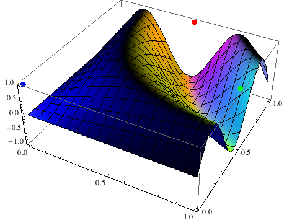
Start with an example plot, motivated by this StackExchange post:

lightSources = {{"Point", Red, {1/2, 1, 1}}, {"Point", 
    Green, {1, 1/2, 1}}, {"Point", Blue, {0, 0, 1}}};
pl = Show[
  Plot3D[Sin[x*y*Pi^2], {x, 0, 1}, {y, 0, 1}, 
   Lighting -> lightSources], 
  Graphics3D[{PointSize[Large], 
    Point[lightSources[[All, 3]], 
     VertexColors -> lightSources[[All, 2]]]}]]
      

The only format I found that preserved the information about the light sources is x3d, so we use Export["pl1.x3d", pl]; and start up Blender.

I'm using Blender 2.60 here. In version 2.65 I observed a glitch in that I couldn't interact properly with the part of the mesh that describes the surface polygons.

After deleting the default cube and importing pl1.x3d, you see this in the 3D view:

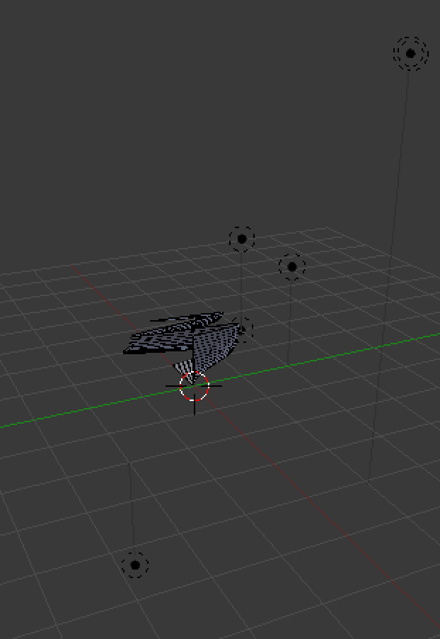
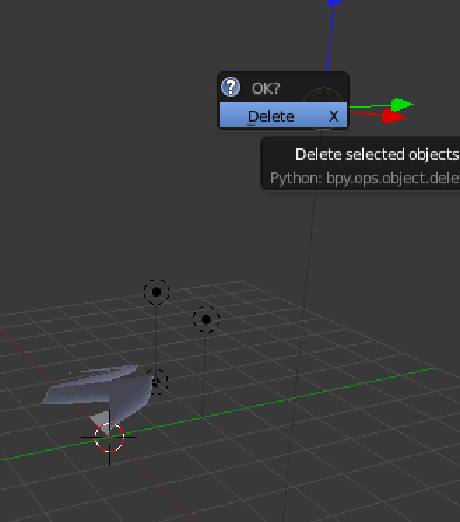
The import contains two mesh objects, and one of them is empty so that it serves no purpose for me. Here I've selected it and pressed x to delete it:

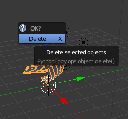
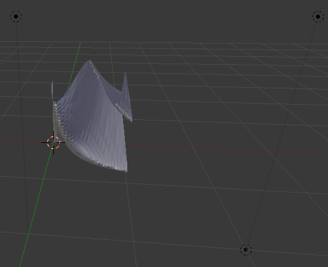
After that's done, the polygons are revealed:

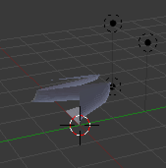
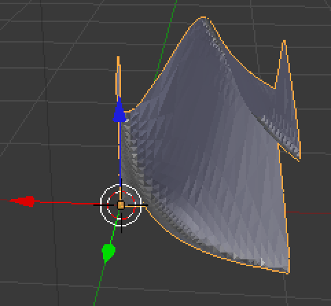
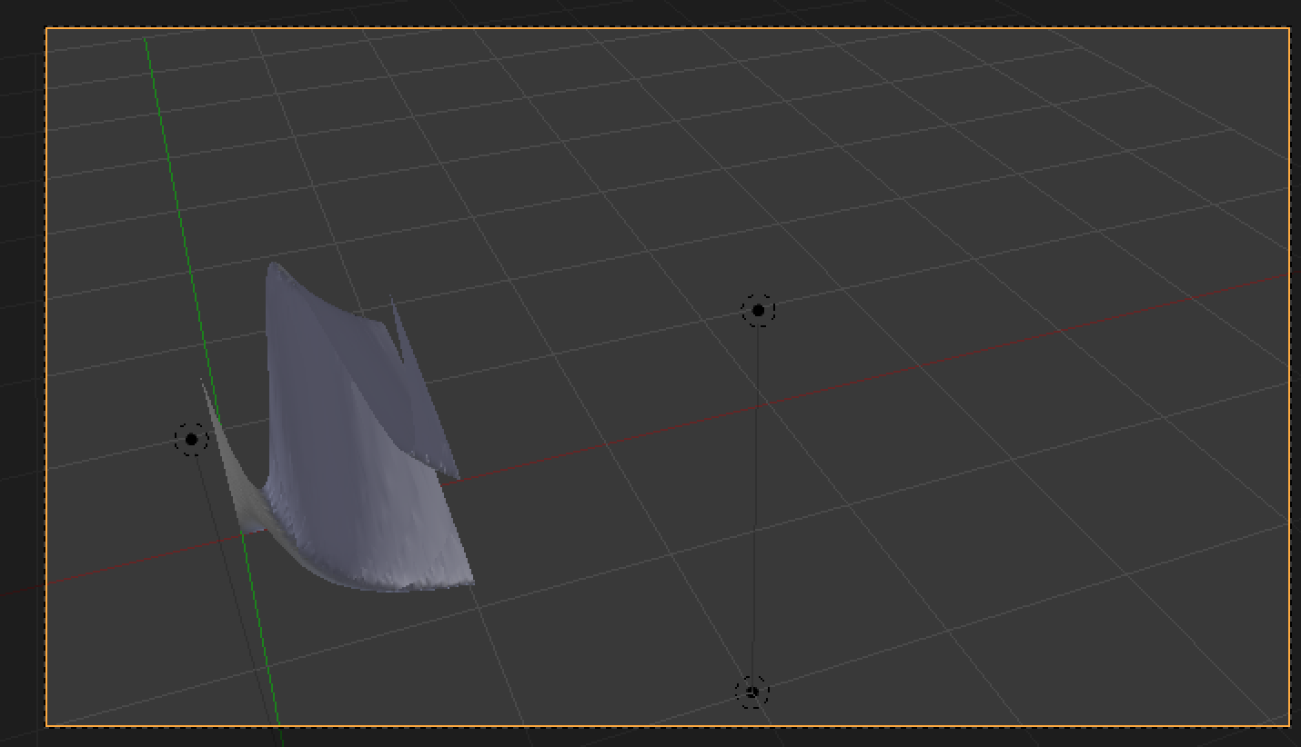
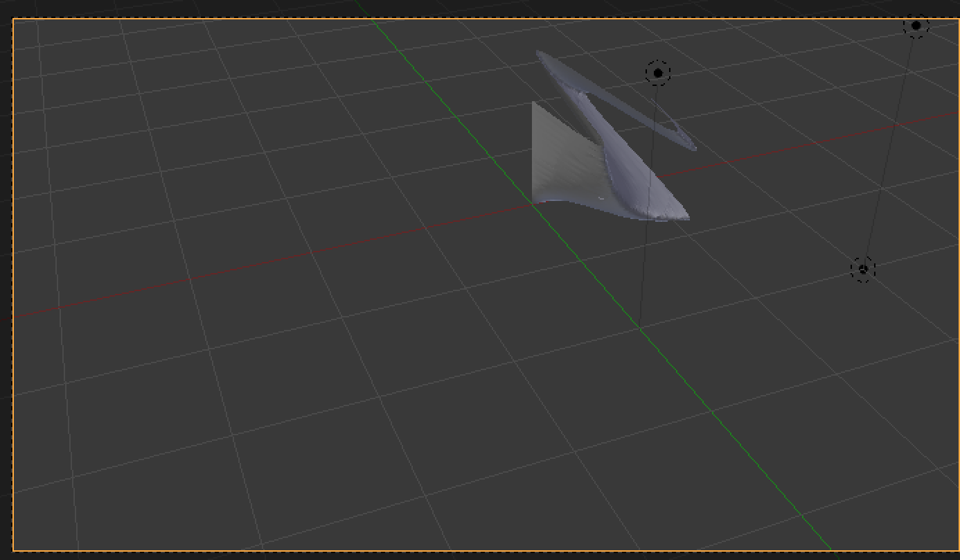
Next, I delete the unwanted light sources of the default scene by selecting each and pressing x:

The remaining light sources are indicated by the black points, but we also see that the polygons are by default displayed flat:

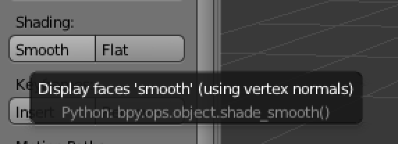
So the next step is to set the surface to smooth (under "shading" in the object properties after you select the surface in the obvect view):

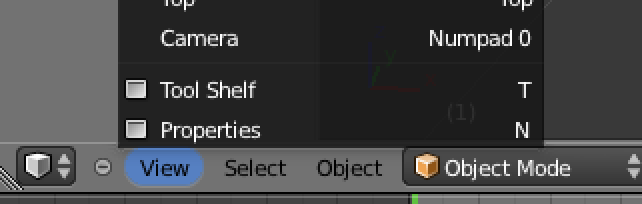
Since the camera position is that of the default scene, we have to move it and rotate (using, e.g., g and r commands), until the camera view shows an acceptable persepctive. This view is selected in the menu shown here:

With this, we're ready to render, by pressing Image here

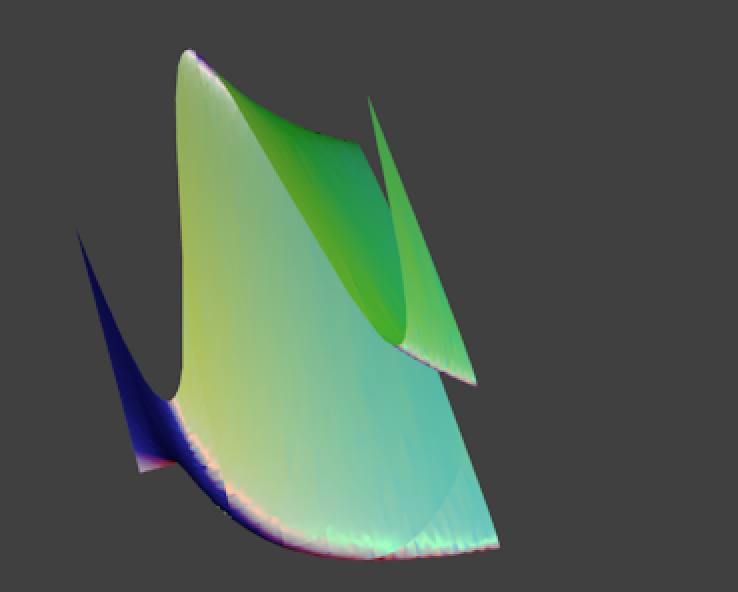
and get the following output:

To see the shadows cast by the shape on iself, move the camera correspondingly:

Now render a second time to see this:

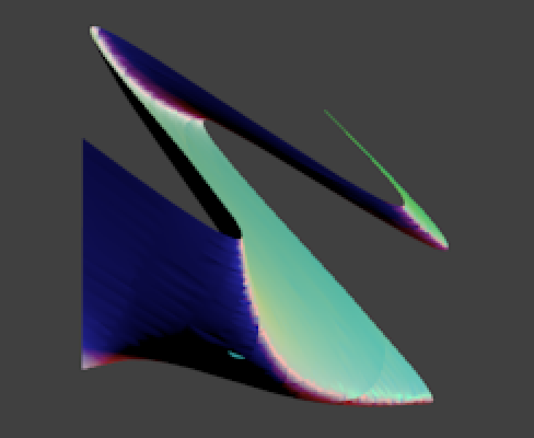
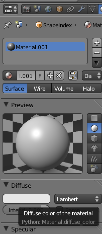
A small bright fleck in the dark region indicates that the polygons for the surface aren't perfect. This could be changed in Mathematica 3d plot settings. Additional fine-tuning could be done by changing the diffuse and specular properties of the surface in the Materials panel (first click the sphere at the top right in the screenshot here, to see the menu appear):

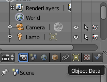
If it's necessary to adjust the light source properties, select the lamp in the object view and check its properties (that's the yellow icon near the bottom below):

---

noeckel@uoregon.edu

Last modified: Wed Jan 16 22:39:02 PST 2013