This is the HTML version of a Mathematica notebook, written for version 8 and 9. You can copy and paste the following into a notebook as literal plain text. For the motivation and further discussion of this notebook, see "Mathematica density and contour Plots with rasterized image representation".
This version has been updated to allow the option PlotLegends which was introduced in version 9.
When regular ContourPlot and ListContourPlot graphics are exported as PDF, the shading appears as a patchwork of polygons with distracting mesh lines. Also, it is impossible to make the contour shading translucent without introducing the mesh line artifacts. Instead of trying to pick out the mesh lines after the fact and adjusting their color or opacity, I decided that the polygons themselves are too much of a nuisance because they also bloat the PDF file.
The two functions rasterContourPlot and rasterListContourPlot defined here work essentially the same as ContourPlot and ListContourPlot, except that the contour shading is represented by a single rasterized image. Because an image can also have an alpha channel (transparency), there is one additional option you can specifiy:
"ShadingOpacity" -> 0 ... 1
rasterContourPlot[f_, rx_, ry_, opts : OptionsPattern[]] := Module[
  {
   img,
   cont,
   contL,
   plotRangeRule,
   contourOptions,
   frameOptions,
   rangeCoords
   },
  contourOptions =
   Join[
    FilterRules[{opts},
     FilterRules[
      Options[ContourPlot],
      Except[{Background, Frame, Axes}]
      ]
     ],
    {Frame -> None, Axes -> None}
    ];
  contL = ContourPlot[f, rx, ry,
    Evaluate@Apply[Sequence, contourOptions]
    ];
  cont = First[Cases[{contL}, Graphics[__], Infinity]];
  img = Rasterize[
    Graphics[
     GraphicsComplex[cont[[1, 1]], cont[[1, 2, 1]]],
     PlotRangePadding -> None, ImagePadding -> None,
     Options[cont, PlotRange]
     ], "Image",
    ImageSize -> With[
      {size =
        Total[{2, 0} (ImageSize /. {opts}) /.
          {ImageSize ->
            CurrentValue[ImageSize]}]},
      If[NumericQ[size],
       size,
       First[WindowSize /. Options[EvaluationNotebook[]]]
       ]
      ]
    ];
  plotRangeRule = FilterRules[Quiet@AbsoluteOptions[cont], PlotRange];
  rangeCoords = Transpose[PlotRange /. plotRangeRule];
  frameOptions = Join[
    FilterRules[{opts},
     FilterRules[Options[Graphics],
      Except[{PlotRangeClipping, PlotRange}]
      ]
     ],
    {plotRangeRule, Frame -> True, PlotRangeClipping -> True}
    ];
  If[Head[contL] === Legended, Legended[#, contL[[2]]], #] &@
  Show[
   Graphics[
    {
     Inset[
      Show[
       SetAlphaChannel[img,
        "ShadingOpacity" /. {opts} /. {"ShadingOpacity" -> 1}
        ], AspectRatio -> Full
       ],
      rangeCoords[[1]], {0, 0}, rangeCoords[[2]] - rangeCoords[[1]]
      ]
     },
    PlotRangePadding -> None
    ],
   Graphics[
    GraphicsComplex[cont[[1, 1]], cont[[1, 2, 2]]],
    PlotRangePadding -> None,
    ImagePadding -> None
    ],
   Evaluate@Apply[Sequence, frameOptions]
   ]
  ]
rasterListContourPlot[pList_, opts : OptionsPattern[]] := Module[
  {img,
   cont,
   contL,
   plotRangeRule,
   contourOptions,
   frameOptions,
   rangeCoords
   },
  contourOptions = Join[
    FilterRules[{opts},
     FilterRules[Options[ListContourPlot],
      Except[{Background, Frame, Axes}]]
     ],
    {Frame -> None, Axes -> None}
    ];
  contL = ListContourPlot[pList,
    Evaluate@Apply[Sequence, contourOptions]
    ];
  cont = First[Cases[{contL}, Graphics[__], Infinity]];
  img = Rasterize[
    Graphics[
     GraphicsComplex[cont[[1, 1]], cont[[1, 2, 1]]],
     PlotRangePadding -> None, ImagePadding -> None,
     Options[cont, PlotRange]
     ], "Image",
    ImageSize -> With[{size =
        Total[{2, 0} (ImageSize /. {opts}) /. {ImageSize ->
            CurrentValue[ImageSize]}]},
      If[NumericQ[size],
       size,
       First[WindowSize /. Options[EvaluationNotebook[]]]
       ]
      ]
    ];
  plotRangeRule = FilterRules[AbsoluteOptions[cont], PlotRange];
  rangeCoords = Transpose[PlotRange /. plotRangeRule];
  frameOptions = Join[
    FilterRules[{opts},
     FilterRules[Options[Graphics],
      Except[{PlotRangeClipping, PlotRange}]]
     ],
    {plotRangeRule, Frame -> True, PlotRangeClipping -> True}
    ];
  If[Head[contL] === Legended, Legended[#, contL[[2]]], #] &@
  Show[
   Graphics[
    {
     Inset[Show[
       SetAlphaChannel[img,
        "ShadingOpacity" /. {opts} /. {"ShadingOpacity" -> 1}],
       AspectRatio -> Full],
      rangeCoords[[1]], {0, 0}, rangeCoords[[2]] - rangeCoords[[1]]
      ]
     },
    PlotRangePadding -> None
    ],
   Graphics[
    GraphicsComplex[cont[[1, 1]], cont[[1, 2, 2]]]
    ],
   Evaluate@Apply[Sequence, frameOptions]
   ]
  ]
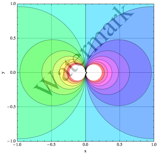
The ability to set an opacity for the contour shading makes it easy to add additional material in the Prolog of the graphic:
rasterContourPlot[Re[1/(x + I y)], {x, -1, 1}, {y, -1, 1},
 GridLines -> Automatic, Contours -> 15, "ShadingOpacity" -> .5,
 ColorFunction -> Hue,
 Prolog ->
  Rotate[Text[
    Style["Watermark", FontSize -> 64,
     GrayLevel[.5]], {0, .3}], π/4], FrameLabel -> {"x", "y"},
 ImageSize -> Automatic]
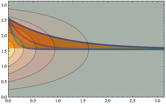
Let's define a list of data that describes a 2D height field:
grid = Transpose[
  Table[Sum[((-1)^n*(Sin[(2*n + 1)*y]/(2*n + 1)^2))/
     E^((2*n + 1)*x), {n, 0, 10}], {x, 0, π, π/24},
   {y, 0, π, π/24}]];
Here we create a contour plot of the data, using rasterized shading with 50% opacity (it will be displayed below):
plot = rasterListContourPlot[grid,
   DataRange -> {{0, π}, {0, π}},
   ColorFunction -> "FallColors", InterpolationOrder -> 2,
   "ShadingOpacity" -> .5, PlotRange -> All];
What if we want to superimpose this with another plot?
plot2 = Plot[
   Evaluate@Table[π/2 + E^(-(2 n + 1) x), {n, 0, 4}], {x,
    0, π}, PlotRangePadding -> 0, PlotRange -> All,
   PlotStyle -> Thickness[.01], Filling -> Axis,
   FillingStyle -> Orange];
To superimpose them, I put the contour plot on top to show that it is indeed translucent:
Show[plot2, plot, Axes -> None, Frame -> True]