(which we measure with respect to the surface normal) and relative
refractive index n. In particular, RFresnel drops significantly below the critical angle for total
internal reflection,
(which we measure with respect to the surface normal) and relative
refractive index n. In particular, RFresnel drops significantly below the critical angle for total
internal reflection, |
An overview is provided over the physics of dielectric microcavities with non-paraxial mode structure; examples are microdroplets and edge-emitting semiconductor microlasers. Particular attention is given to cavities in which two spatial degrees of freedom are coupled via the boundary geometry. This generally necessitates numerical computations to obtain the electromagnetic cavity fields, and hence intuitive understanding becomes difficult. However, as in paraxial optics, the ray picture shows explanatory and predictive strength that can guide the design of microcavities. To understand the ray-wave connection in such asymmetric resonant cavities, methods from chaotic dynamics are required. |
Maxwell’s equations of electrodynamics exemplify how the beauty of a theory is captured in the formal simplicity of its fundamental equations. Precisely for this reason, they also illustrate that physical insight cannot be gleaned from the defining equations of a theory per se unless we understand how these equations are solved in practice. In optics, one powerful approach to this challenge is the short-wavelength approximation leading to the ray picture. Rays are the solutions to Fermat’s variational principle, which in particular implies the laws of reflection and refraction at dielectric interfaces. As soon as one makes the transition from wave physics to this classical domain, concepts such as “trajectory”, “phase space” and “diffusion” become meaningful. In this chapter, special attention will be devoted to the classical phenomenon of chaos in the ray dynamics of small optical cavities, i.e., a sensitive dependence of the ray traces on initial conditions. The main implication for the corresponding wave equation is that it cannot be reduced to a set of mutually independent ordinary differential equations, e.g., by separation of variables. Even when only a few degrees of freedom are present in the system, their coupling then makes it impossible to label the wave solutions by a complete set of “quantum numbers” (e.g., longitudinal and transverse mode numbers). Such a problem is called non-integrable; this classification is due to Poincaré and applies both to rays and waves [1]. Integrable systems are characterized by a complete set of “good quantum numbers”, as will be illustrated in section 9
Microcavities can be broadly categorized into active (light emitting) and passive systems. In active devices, such as lasers, radiation is generated within the cavity medium, without any incident radiation at the same frequency; the cavity provides feedback and (in combination with a gain medium) sets the emission wavelength [2]. Some of the important properties that characterize a light emitting cavity are emission spectra, emission directivity, output energy, noise properties and lasing thresholds. Examples for passive systems are filters, multiplexers and other wavelength-selective optical components; their functionality relies on coupling to waveguides or freely propagating waves in their vicinity. To characterize and operate passive cavities, one is interested in transmission and reflection coefficients, i.e., in the resonator as a scatterer.
The two basic types of experiment, emission and scattering, for a given cavity geometry are intimately connected because they both probe its mode structure. The concept of modes in microcavities will be made more precise in section 8; as a working definition, let us denote as modes all electromagnetic excitations of the cavity which show up as peak structure in scattering or emission spectra and are caused by constructive interference in the resonator.
Nonintegrable cavities introduce added freedom into the design of novel optical components, especially when we apply results from the field of quantum chaos, in which modern quasiclassical methods are of central importance [3, 4, 5, 6, 7, 8, 9]. The term “quantum” in “quantum chaos” relates to the fact that cavity modes are discrete as a consequence of the constructive interference requirement mentioned above; the term “chaos” refers to a degree of complexity in the ray picture which renders inapplicable all simple quantization schemes such as the paraxial method.
The optics problem we are addressing is not one of “quantum optics”, but of the quantized (i.e., discrete) states of classical electrodynamics in spatially confined media. By quasiclassics, we therefore mean the short-wavelength treatment of the classical electromagnetic field. Confusion should be avoided between quasiclassics as defined here, and the semiclassical treatment of light in the matter-field interaction, which couples quantum particles to the electromagnetic field via the classical (vector) potentials: how we obtain the modes of a cavity (e.g., quasiclassically), should be distinguished from how we use them (e.g., as a basis in quantum optical calculations). Our main emphasis in this chapter will be on the “how” part of the problem, but the wealth of physics contained in these modes themselves points to novel applications as well. Having made this clarification, we henceforth use the term “semiclassics” synonymously with “quasiclassics” as defined above.
Many of the microcavities which are the subject of this chapter employ “mirrors” of a simple but efficient type: totally reflecting abrupt dielectric interfaces between a dielectric body and a surrounding lower-index medium. Resonators occurring in nature, such as droplets or microcrystals, use this mechanism to trap light. This allows us to draw parallels between nature and a variety of technologically relevant resonator designs that are based on the same confinement principle. A recurring theme in numerous systems is the combination of total internal reflection (TIR) with a special type of internal trajectory that skips along the boundary close to grazing incidence: the “whispering-gallery” (WG) phenomenon, named after an acoustic analogue in which sound propagates close to the curved walls of a circular hall without being audible in its center [10, 11]. An example for the use of the WG effect in cavity ring-down spectroscopy is reported in Ref. [12]. A WG cavity can provide the low loss needed to reduce noise and improve resolution in the detection of trace species; the trace chemicals are located outside the cavity and couple to the internal field by frustrated total internal reflection, or evanescent fields. In this section, we review Fresnel’s formulas before introducing the WG modes. This provides the basis for sections 9 - 16
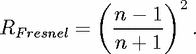
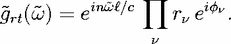
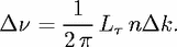
In the ray picture, the Fresnel reflectivity, RFresnel, of a dielectric interface depends on the
angle of incidence (which we measure with respect to the surface normal) and relative
refractive index n. In particular, RFresnel drops significantly below the critical angle for total
internal reflection,
 | (1) |
 | (2) |
 | (3) |
 does not enter the Fresnel formulas, internal reflection can
be classified as a “classical” phenomenon which can be understood based on Fermat’s
principle.
This should be contrasted with the intrinsic frequency dependence of Bragg reflection – the
other widespread mechanism for confining light in dielectrics. From an engineering point of
view, Bragg reflectors are challenging to realize for lateral confinement. In particular for
low-index materials, high-reflectivity windows (stop bands) are direction- and frequency
dependent with narrow bandwidth. TIR, on the other hand, is broad-band and technologically
simple.
does not enter the Fresnel formulas, internal reflection can
be classified as a “classical” phenomenon which can be understood based on Fermat’s
principle.
This should be contrasted with the intrinsic frequency dependence of Bragg reflection – the
other widespread mechanism for confining light in dielectrics. From an engineering point of
view, Bragg reflectors are challenging to realize for lateral confinement. In particular for
low-index materials, high-reflectivity windows (stop bands) are direction- and frequency
dependent with narrow bandwidth. TIR, on the other hand, is broad-band and technologically
simple.
At higher orders of , wavelength-dependent corrections to Fresnel’s formulas do arise
because TIR is truly total only for a plane wave incident on an infinite and flat interface. The
latter does not hold for boundaries with finite curvature or even sharp corners, and similarly
in cases where the incident beam has curved wavefronts, as in a Gaussian beam
[13, 14, 15, 16]. The physical reason for radiation leakage in these situations is that light
penetrates the dielectric interface to some distance which depends exponentially on , as in
quantum-mechanical tunneling. This allows coupling to the radiation field outside the cavity
[13, 14].
The analogy to quantum mechanics rests on the similarity between the Schrödinger and
the Helmholtz equation for the field  ,
,
 | (4) |
 , z. The circular
cylinder and sphere are the two main representatives of this small class [7, 17] of
integrable dielectric scattering problems. The analytic solution, due to Lorentz and
Mie, of Maxwell’s vector wave equations for a dielectric sphere, has a long history
[17, 18, 19, 20, 13, 14]). It finds application in a wide range of different optical
processes, ranging from elastic scattering by droplets to nonlinear optics [25] and to
cavity quantum electrodynamics [21, 22, 23]. Similarly, dielectric cylinders are used,
e.g., as models for atmospheric ice particles [24] or edge-emitting microdisk and
micropillar lasers [26, 27, 28]. Because of rotational symmetry, the ray motion in a
sphere is always confined to a fixed plane. By contrast, rays in a cylinder can spiral
along the axis [29, 30], but the propagation becomes planar if the incident wave is
aligned to be perpendicular to the cylinder axis. Similar symmetry arguments make it
possible to find analytic solutions in concentrically layered dielectrics or ring resonators
[31, 32, 33].
Each time a degree of freedom can be separated due to symmetry, the effective
dimensionality of the remaining wave equation is reduced by one – in the above examples one
finally arrives at an ordinary (one dimensional) equation for the radial coordinate. Even
without symmetry properties such as in the sphere or cylinder, one often finds approximate
treatments by which such a reduction from three to fewer dimensions can be justified: in fact,
in integrated optics, most functions are performed by planar optical devices, for which the
mode profile in the vertical direction can be approximately separated from the wave equation
in the horizontal plane, leaving a two-dimensional problem. For a discussion of methods
exploiting this assumption (e.g. the effective-index method), the reader is referred to the
literature [34].
, z. The circular
cylinder and sphere are the two main representatives of this small class [7, 17] of
integrable dielectric scattering problems. The analytic solution, due to Lorentz and
Mie, of Maxwell’s vector wave equations for a dielectric sphere, has a long history
[17, 18, 19, 20, 13, 14]). It finds application in a wide range of different optical
processes, ranging from elastic scattering by droplets to nonlinear optics [25] and to
cavity quantum electrodynamics [21, 22, 23]. Similarly, dielectric cylinders are used,
e.g., as models for atmospheric ice particles [24] or edge-emitting microdisk and
micropillar lasers [26, 27, 28]. Because of rotational symmetry, the ray motion in a
sphere is always confined to a fixed plane. By contrast, rays in a cylinder can spiral
along the axis [29, 30], but the propagation becomes planar if the incident wave is
aligned to be perpendicular to the cylinder axis. Similar symmetry arguments make it
possible to find analytic solutions in concentrically layered dielectrics or ring resonators
[31, 32, 33].
Each time a degree of freedom can be separated due to symmetry, the effective
dimensionality of the remaining wave equation is reduced by one – in the above examples one
finally arrives at an ordinary (one dimensional) equation for the radial coordinate. Even
without symmetry properties such as in the sphere or cylinder, one often finds approximate
treatments by which such a reduction from three to fewer dimensions can be justified: in fact,
in integrated optics, most functions are performed by planar optical devices, for which the
mode profile in the vertical direction can be approximately separated from the wave equation
in the horizontal plane, leaving a two-dimensional problem. For a discussion of methods
exploiting this assumption (e.g. the effective-index method), the reader is referred to the
literature [34].
One of the advantages of reducing the cavity problem to two degrees of freedom is that polarizations can approximately be decoupled into TE and TM. The resulting wave equations are then scalar, with the polarization information residing in the continuity conditions imposed on the fields at dielectric interfaces. Therefore, the fields are formally obtained as solutions of Eq. (4) in two dimensions. This scalar problem is the starting point for our analysis. In the absence of absorption or amplification, the index n(r) which defines our microcavity is real-valued, and approaches a constant (taken here as n = 1 for air) outside some finite three-dimensional domain corresponding to the cavity.
|
|
The wave solutions shown in Fig. 2 show field intensity extending to the exterior of the
cavity because the dielectric interface is “leaky”. In general, such a calculation must be
performed numerically; we shall discuss the definition and emission properties of these leaky
modes further below, in section 4 For now, we are only concerned with the internal intensity
patterns. The reader will recognize a strong similarity between the “bouncing-ball” mode and a
higher-order transverse Gauss-Hermite beam; this arises because the ray motion corresponding
to this mode is a stable oscillation between the flat sides of the cavity. The analytic transverse
form of the bouncing-ball beam in the ellipse is however not a Gaussian, but a Mathieu
function. The caption of Fig. 2 gives the linewidth  of the two types of modes,
indicating that the WG resonance is almost an order of magnitude narrower than
the bouncing-ball mode, despite the twofold higher refractive index used in Fig. 2
(b).
of the two types of modes,
indicating that the WG resonance is almost an order of magnitude narrower than
the bouncing-ball mode, despite the twofold higher refractive index used in Fig. 2
(b).
The ellipse has been chosen as an example because it is integrable in the limit of no leakage. Other oval deformations of the circle do not have this simplifying property. However, families of WG ray trajectories have been proven [39] to exist in any sufficiently smooth and oval enclosure, provided that its curvature is nowhere zero. This makes WGMs a very robust phenomenon of general convex oval cavities. Before we discuss in more detail the relation between the ray picture and the internal structure of the resonator modes, we now turn to some general considerations on what allows us to define the modes of an open cavity.
WGMs are not infinitely long-lived even in an ideal dielectric cavity, as we saw in the finite
linewidths of Fig. 1. In fact, for a finite, three-dimensionally confined dielectric body, all
solutions to Eq. (4) are extended to infinity, forming a continuous spectrum. A basis of
eigenfunctions is given by the scattering states, consisting of an incoming wave ψin that is
elastically scattered by the dielectric microstructure of index n(r) into an outgoing wave ψout. In
the asymptotic region where n = 1, the relation between incoming and outgoing waves
is mediated by the scattering operator S, known from quantum scattering theory
[40], to which the electromagnetic resonator problem is conceptually analogous.
The S-matrix formalism has long been in use in microwave technology as well as
optics [41]: A matrix representation is obtained by defining basis states | > (|
> (| >) in
which the asymptotic incoming (resp., outgoing) fields can be expanded; one has
>) in
which the asymptotic incoming (resp., outgoing) fields can be expanded; one has
Only the properties of the index profile, not of the particular incoming wave, enter S. For a review of scattering theory see, e.g., [42]. As was seen in Fig. 1, the actual cavity modes in this continuum of scattering states are revealed if we measure the scattering of light as a function of wavenumber k. The amplitude of the scattered field shows resonant structure at discrete values of k which do not depend on the detailed spatial form of the exciting field ψin. These resonances are caused by poles of S in the complex k plane, and are a characteristic of the microcavity itself. In Eq. (5), we note that a pole of S admits nonvanishing ψout in the absence of any incoming waves, ψin = 0. In these solutions at complex k, also known as the quasibound states, we have finally found a proper definition of what we simply called “cavity modes” earlier.
A well-known example is the linear two-mirror (Fabry-Perot) cavity [2]. Its resonances are
easily obtained within physical optics by writing the transmission of an incident ray as a
geometric series over multiple round trips. In each round trip, the amplitude of a ray in the
cavity accrues a factor r1r2 exp(ink  + i1 + i2), where is the round-trip path length. We
have split the amplitude reflectivities at the individual reflections = 1, 2 into modulus r
+ i1 + i2), where is the round-trip path length. We
have split the amplitude reflectivities at the individual reflections = 1, 2 into modulus r and phase . Attenuation comes from r < 1 ( = 1, 2 in the two-mirror case). The refractive
index n in the cavity is real, as stated below Eq. (4), and the wave number k is measured in
free space. The transmitted amplitude Ttotal is obtained by summing this over all repetitions,
and phase . Attenuation comes from r < 1 ( = 1, 2 in the two-mirror case). The refractive
index n in the cavity is real, as stated below Eq. (4), and the wave number k is measured in
free space. The transmitted amplitude Ttotal is obtained by summing this over all repetitions,
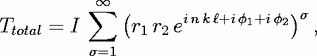 | (6) |
 rt(
rt( ), with the round-trip
“gain”
), with the round-trip
“gain”
 | (7) |
runs from 1 to 2. Whenever  rt comes close to 1, the resonator exhibits a
transmission peak. The equality
rt comes close to 1, the resonator exhibits a
transmission peak. The equality  rt(
rt( ) = 1 can be satisfied only if we admit complex
frequencies,
) = 1 can be satisfied only if we admit complex
frequencies,  ≡ω+iγ, and choose for the imaginary part
 | (8) |
 determines the resonance linewidth. Were we to look at the
complex-frequency solution directly and reinstate the time dependent factor exp(i
determines the resonance linewidth. Were we to look at the
complex-frequency solution directly and reinstate the time dependent factor exp(i t) that
accompanied the original wave equation, the field at every point in space would decay with a
factor exp(-t). An interpretation of this can be given in the ray picture: for a ray
launched inside the cavity, the field is attenuated by a factor r1 r2 in each round
trip; after time t, the number of round trips is ct/, leading to the exponential law
t) that
accompanied the original wave equation, the field at every point in space would decay with a
factor exp(-t). An interpretation of this can be given in the ray picture: for a ray
launched inside the cavity, the field is attenuated by a factor r1 r2 in each round
trip; after time t, the number of round trips is ct/, leading to the exponential law
 | (9) |
and of a multichannel scattering process to a sum over all possible ray paths starting in
channel and ending in :
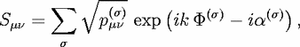 | (10) |
 parameterizes the family of ray trajectories leading from incoming channel to
outgoing channel , just as in Eq. (6).
parameterizes the family of ray trajectories leading from incoming channel to
outgoing channel , just as in Eq. (6).  (
( ) is a phase shift acquired by the rays as they
encounter caustics and interface reflections along their path. The phase shift k
) is a phase shift acquired by the rays as they
encounter caustics and interface reflections along their path. The phase shift k () is the
generalization of the dynamical phase k in the linear example, and pμν(σ) is the transition
probability, corresponding to the product of reflection and transmission coefficients in our
two-mirror example. For a cavity defined by Fresnel reflection, pμν(σ) can to lowest approximation
be determined purely within ray optics.
The virtue of Eq. (10) is that it points the way from geometric optics to wave
optics even in systems where the ray paths are not as easily enumerated as in the
Fabry-Perot cavity. The Fabry-Perot cavity discussed above is an example where
Eq. (10) in fact yields exact results, because only plane-wave propagation is involved.
Although corrections to this quasiclassical formula are necessary in more complicated
cavity geometries, Eq. (10) makes it plausible that ray considerations are a powerful
tool for understanding quasibound states in many open systems. In this spirit of
ray-based scattering theory, we can ask how to extract the quasibound states as
poles of the physical-optics expression Eq. (10). This means we want to generalize
the logical transition (illustrated for the Fabry-Perot cavity) from a transmission
amplitude determined by Eq. (7) to an internal ray loop with attenuation given by
Eq. (9). Thus, the original scattering problem should be replaced by a Monte-Carlo
simulation of a suitable ensemble of rays inside the resonator, and the internal ray
dynamics suffers dissipation owing to the openness of the cavity. Several technical
problems make it difficult to carry out this idea in a general cavity: the first question
is what would be the proper choice of initial conditions for a ray ensemble in a
two-dimensional cavity such as the ellipse of Fig. 2. The answer is provided by
quasiclassical quantization conditions that put some constraint on the ray paths to be
used in the ray calculation. Employing a strategy along these lines, it is possible to
predict not only the decay rate of a quasibound state as in Eq. (9), but also the
directionality of the emitted radiation [51]. This will be expounded in sections 11 and
14.
() is the
generalization of the dynamical phase k in the linear example, and pμν(σ) is the transition
probability, corresponding to the product of reflection and transmission coefficients in our
two-mirror example. For a cavity defined by Fresnel reflection, pμν(σ) can to lowest approximation
be determined purely within ray optics.
The virtue of Eq. (10) is that it points the way from geometric optics to wave
optics even in systems where the ray paths are not as easily enumerated as in the
Fabry-Perot cavity. The Fabry-Perot cavity discussed above is an example where
Eq. (10) in fact yields exact results, because only plane-wave propagation is involved.
Although corrections to this quasiclassical formula are necessary in more complicated
cavity geometries, Eq. (10) makes it plausible that ray considerations are a powerful
tool for understanding quasibound states in many open systems. In this spirit of
ray-based scattering theory, we can ask how to extract the quasibound states as
poles of the physical-optics expression Eq. (10). This means we want to generalize
the logical transition (illustrated for the Fabry-Perot cavity) from a transmission
amplitude determined by Eq. (7) to an internal ray loop with attenuation given by
Eq. (9). Thus, the original scattering problem should be replaced by a Monte-Carlo
simulation of a suitable ensemble of rays inside the resonator, and the internal ray
dynamics suffers dissipation owing to the openness of the cavity. Several technical
problems make it difficult to carry out this idea in a general cavity: the first question
is what would be the proper choice of initial conditions for a ray ensemble in a
two-dimensional cavity such as the ellipse of Fig. 2. The answer is provided by
quasiclassical quantization conditions that put some constraint on the ray paths to be
used in the ray calculation. Employing a strategy along these lines, it is possible to
predict not only the decay rate of a quasibound state as in Eq. (9), but also the
directionality of the emitted radiation [51]. This will be expounded in sections 11 and
14.
We now discuss the significance of complex frequencies in Eqs. (4) and (5). This will highlight
the relation between quasibound states and the observable cavity response to an external field
or pump signal, which is of particular interest in spectroscopy. In Eq. (4), the wavenumber
only appears in the form of a product nk, so that an imaginary part in  ≡k + iκ≡
 /c can
immediately be re-interpreted as part of a complex refractive index ñ at real k, setting
/c can
immediately be re-interpreted as part of a complex refractive index ñ at real k, setting
 | (11) |
> 0: a plane wave would have the form
exp(i t - iñkx), which grows in the propagation direction. From Eq. (11) it follows that
quasibound states appear naturally as approximate solutions for the lasing modes of a
microlaser with a homogeneous gain medium [52]. For a physical understanding of lasers
[53], the openness of the system as contained in the quasibound state description is
essential.
When a cavity is excited with a pulse, on the other hand, we are not looking for
steady-state solutions but for transients. As we noted below Eq. (9), quasibound states
describe such a decay process. These non-stationary states are exploited in many fields, e.g.
nuclear physics (where they are called “Gamov states”), and their properties are well-known
[54, 55]. One peculiar property that may cause confusion is that they formally diverge in the
far field, as can be seen by noting that the outgoing wave in Eq. (5) obeys the
radiation boundary condition, which in the continuation to complex frequency reads
t - iñkx), which grows in the propagation direction. From Eq. (11) it follows that
quasibound states appear naturally as approximate solutions for the lasing modes of a
microlaser with a homogeneous gain medium [52]. For a physical understanding of lasers
[53], the openness of the system as contained in the quasibound state description is
essential.
When a cavity is excited with a pulse, on the other hand, we are not looking for
steady-state solutions but for transients. As we noted below Eq. (9), quasibound states
describe such a decay process. These non-stationary states are exploited in many fields, e.g.
nuclear physics (where they are called “Gamov states”), and their properties are well-known
[54, 55]. One peculiar property that may cause confusion is that they formally diverge in the
far field, as can be seen by noting that the outgoing wave in Eq. (5) obeys the
radiation boundary condition, which in the continuation to complex frequency reads
 | (12) |
of  causes exponential growth with r. However, grouping
together the exponential dependences on position and time, the amplitude of the quasibound
state is controlled by the factor
causes exponential growth with r. However, grouping
together the exponential dependences on position and time, the amplitude of the quasibound
state is controlled by the factor
 | (13) |

 therefore has nothing unphysical, provided causality is taken into account:
within the ring-down time 1/ of the cavity, the maximum distance to which we
can extend measurements of the radiated field is of order R ~ c/ = 1/. In this
range, r < R, the decaying pre-exponential factors dominate over the exponential r
dependence.
Equation (11) represents a level of approximation which does not take microscopic
properties of the light-emitting medium into account. However, it forms a starting point which
emphasizes the effect of the resonator boundaries on the mode structure from the outset; an
effect that becomes essential as the cavity size decreases. If we allow the polarization P,
which in Maxwell’s wave equation effects the coupling between matter and field,
to become a function of position, and possibly acquire a nonlinear dependence on
the electric field, then it turns out that the quasibound states of the homogeneous
medium, discussed above, are nevertheless a convenient basis in which to describe the
emission and mode coupling caused by P. To make this plausible, recall that any given
electromagnetic cavity field can be expanded in an integral over the scattering states scat of
Eq. (5) as a function of k; these are the “modes of the universe” in the presence of the
cavity. To evaluate such an integral, one can extend the integration contour into the
complex plane and apply the residue theorem. The integral is then converted to a
sum over those k at which the integrand has a pole. But the poles of the scattering
states are just the poles of the S matrix, i.e. the quasibound states. For details
of these arguments, the reader should see Ref. [54]. The radiation from a source
distribution d(r) is obtained directly by summing up those quasibound states which lie
in the spectral interval of interest, weighted according to their overlap with the
distribution d(r), and with an energy denominator that makes sharp resonances
contribute more strongly than broad ones. In particular, for small cavities where the free
spectral range is large and the linewidths are small, the emission properties are
determined by the spatial form and temporal behavior of individual quasibound
states.
therefore has nothing unphysical, provided causality is taken into account:
within the ring-down time 1/ of the cavity, the maximum distance to which we
can extend measurements of the radiated field is of order R ~ c/ = 1/. In this
range, r < R, the decaying pre-exponential factors dominate over the exponential r
dependence.
Equation (11) represents a level of approximation which does not take microscopic
properties of the light-emitting medium into account. However, it forms a starting point which
emphasizes the effect of the resonator boundaries on the mode structure from the outset; an
effect that becomes essential as the cavity size decreases. If we allow the polarization P,
which in Maxwell’s wave equation effects the coupling between matter and field,
to become a function of position, and possibly acquire a nonlinear dependence on
the electric field, then it turns out that the quasibound states of the homogeneous
medium, discussed above, are nevertheless a convenient basis in which to describe the
emission and mode coupling caused by P. To make this plausible, recall that any given
electromagnetic cavity field can be expanded in an integral over the scattering states scat of
Eq. (5) as a function of k; these are the “modes of the universe” in the presence of the
cavity. To evaluate such an integral, one can extend the integration contour into the
complex plane and apply the residue theorem. The integral is then converted to a
sum over those k at which the integrand has a pole. But the poles of the scattering
states are just the poles of the S matrix, i.e. the quasibound states. For details
of these arguments, the reader should see Ref. [54]. The radiation from a source
distribution d(r) is obtained directly by summing up those quasibound states which lie
in the spectral interval of interest, weighted according to their overlap with the
distribution d(r), and with an energy denominator that makes sharp resonances
contribute more strongly than broad ones. In particular, for small cavities where the free
spectral range is large and the linewidths are small, the emission properties are
determined by the spatial form and temporal behavior of individual quasibound
states.
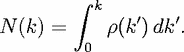
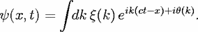
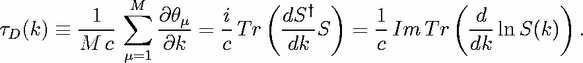
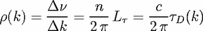
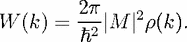
In spectroscopic applications, the quality Q and finesse F of a cavity are important figures of merit. Conventionally, one defines
 | (14) |
 (k). If Q and F were independent of k, then
the total number of cavity modes with wavenumber less or equal to k would be
N(k) = k/FSR = Q/F. The density of states is the k-dependent generalization of the inverse
FSR:
(k). If Q and F were independent of k, then
the total number of cavity modes with wavenumber less or equal to k would be
N(k) = k/FSR = Q/F. The density of states is the k-dependent generalization of the inverse
FSR:
 | (15) |
(k) contains all the information about both Q(k) and F(k).
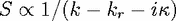
For a dielectric scatterer with sharp boundaries, there is in principle a clear distinction
between “inside” and “outside”. An incoming wave propagates freely outside the dielectric, but
can be trapped inside for some time. Therefore, an incident wave pulse emerges from the
scatterer with a time delay,  D, compared to the time it takes in the absence of the
obstacle (S≡1). The time delay is a continuous function of k, whereas the resonance
decay time 1/ labels discrete poles of the S-matrix. To clarify the relation between
delay time and decay time, consider the simplest case of a one-channel scattering
system, in which in
D, compared to the time it takes in the absence of the
obstacle (S≡1). The time delay is a continuous function of k, whereas the resonance
decay time 1/ labels discrete poles of the S-matrix. To clarify the relation between
delay time and decay time, consider the simplest case of a one-channel scattering
system, in which in  exp(it + ikx) and out exp[it - ikx + i
 (k)]. Here, is
the scattering phase shift, which is related to the (unitary) S-matrix of Eq. (5) by
(k)]. Here, is
the scattering phase shift, which is related to the (unitary) S-matrix of Eq. (5) by
![S(k) = exp[ih(k)].](acad2conv29x.gif) | (16) |
 | (17) |
 (k)|, could be assumed to be either sharply peaked or slowly-varying.
Consider first the case where |(k)| has a narrow peak at some central wavenumber k0; the
opposite limit will be treated in Eq. (27). Then the variation of with k need only be retained
to linear order, yielding
(k)|, could be assumed to be either sharply peaked or slowly-varying.
Consider first the case where |(k)| has a narrow peak at some central wavenumber k0; the
opposite limit will be treated in Eq. (27). Then the variation of with k need only be retained
to linear order, yielding
 | (18) |
0(x,t) the corresponding pulse for θ≡0, i.e. without scattering, then the last
equation means
 | (19) |
D(k) [56, 57]; it is a continuous function of k.
For a general scattering system with M > 1 channels, D(k) is obtained by adding the k -
derivatives of all the phases θμ entering the M eigenvalues exp(i ) of the S matrix:
 | (20) |
r = ckr one has
 | (21) |
describing the linewidth, or the decay rate in Eq. (13) via = c. Then
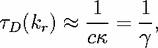 | (22) |
D, as we
can understand from the following (non-rigorous) argument (for more stringent
derivations, see, e.g., [60]): D defines a length scale L ≡cD/n (n is the refractive index)
which is the characteristic distance over which the wave will propagate inside the
scatterer. If we interpret this as the effective “cavity length”, then a mode should
naively be expected when an integer number of wavelengths fits into this length, i.e.,
≡cD/n (n is the refractive index)
which is the characteristic distance over which the wave will propagate inside the
scatterer. If we interpret this as the effective “cavity length”, then a mode should
naively be expected when an integer number of wavelengths fits into this length, i.e.,
 | (23) |
is an integer, and the constant takes into account phase shifts at interface reflections
or caustics. The number of modes that are contained in a small interval  k around k is then
given by the corresponding change in the above equation, which to lowest order in k is
k around k is then
given by the corresponding change in the above equation, which to lowest order in k is
 | (24) |
 | (25) |
 | (26) |
The limit of a well-defined frequency in the wavepacket of Eq. (17) allowed us to assume
that the radiation interacts only with a single quasibound state, leading to the resonant delay
time Eq. (22). On the other hand, if we take |ξ(k)|≡C to be constant, the whole spectrum enters
with equal weight. One could still make the assumption that there is only a single isolated
resonance in the spectrum; then one immediately arrives at the well-known relation
between Lorentzian lineshape and exponential resonance decay: take the resonance
to be at wavenumber kr (it is in fact always accompanied by a partner state [35]
at -kr, but we can ignore it at large enough frequencies); replacing exp(i) = S
in Eq. (17) by Eq. (21), what remains is the Fourier transform of a Lorentzian,
 | (27) |
The two limiting cases of (k) in the wavepacket Eq. (17) are just extremes of the
time-frequency uncertainty relation. Experiments on microcavities have been performed both
in the spectral and time domain. However, there has been only one report of the temporal
nature of an ultra-short optical wavepacket (100 fs pulse, 30 μm short in air) incident on a
pendant-shaped, hanging droplet with an equatorial radius of 520 μm [74]. Such pulses are
spectrally broad but have the intriguing property that their spatial length is much shorter
than the cavity size. Conceptually, the analogy to a well-defined particle trajectory
suggests itself, and hence one looks for ballistic propagation in the cavity. In the
experiment, wavepackets were observed to circulate inside the droplet in the region where
the the WGMs reside; such paths are characteristic of high-order rainbows in that
entry and exit of the light are separated by a large number of internal reflections
[19, 47].
The time-resolved measurement showed that coherent excitation of a large number of
WGMs allows propagation of a short wavepacket along the sphere’s equator for several round
trips without significant decoherence, except for decrease in the wavepacket intensity because
of leakage of the WGMs. The novel aspect of the experiment that enabled the time-resolved
measurements was the use of two-color two-photon-excited Coumarin 510 dye molecules
embedded in the liquid (ethylene glycol) that formed the pendant droplet. The Coumarin
fluorescence (near 510 nm) appears when one wavepacket of 1 and another wavepacket of 2
spatially overlap. Thus, the Coumarin fluorescence acts as a correlator between
wavepackets.
This time-resolved experiment was designed to answer the following questions: (1) does the excitation wavepacket remain intact and ballistic after evanescent coupling with WGMs? (2) after a few round trips, would dispersion cause the wavepacket to broaden? and (3) can the cavity ring down time be observed for those wavepackets that make several round trips? The answers were reached that the shape of excitation wavepacket remained intact, the wavepacket was not broadened after a few round trips, and that cavity ring down was observed for each round trip. This is an extension of the single-mode ring-down determined by Eq. (27).
In particular in the context of cavity ring-down spectroscopy, the usefulness of
time-domain measurements is recognized [75]. There, one deals with very high Q-factors and
their modification by the sample to be studied. Another application of temporal observation is
encountered in microdroplets, where the optical feedback provided by WGMs makes it
possible to reach the threshold for stimulated Raman scattering (SRS). The SRS
spectrum consists of sharp peaks, commensurate with the higher Q WGMs located
within the Raman gain profile. The highest Q value of the WGMs can be determined
either by resolving the narrowest linewidth of the SRS peak or by measuring
the longest exponential decay of the SRS signal after the pump laser pulse is off.
When Q > 105, the decay time = Q/ (where  3 × 10¹⁵ Hz for λ= 620 nm)
becomes a much easier quantity to measure directly because it is longer than 100 ps.
Otherwise, the spectral linewidth ( = /Q) needs to be resolved better than 0.006
nm (for = 600 nm). Cavity decay lifetimes as long as 6.5 ns have been observed
[76].
3 × 10¹⁵ Hz for λ= 620 nm)
becomes a much easier quantity to measure directly because it is longer than 100 ps.
Otherwise, the spectral linewidth ( = /Q) needs to be resolved better than 0.006
nm (for = 600 nm). Cavity decay lifetimes as long as 6.5 ns have been observed
[76].
Having defined the density of modes for the open system in section 6, we can go one step
further and perform the the average  (k) over some finite spectral interval k. The suitable
choice for such an averaging interval should of course contain many spectral peaks. Two
relevant examples where an average spectral density is of use are the Thomas-Fermi model of
the atom [77] and Planck’s radiation law. The latter shall serve as a motivation for
some further discussion of the average
(k) over some finite spectral interval k. The suitable
choice for such an averaging interval should of course contain many spectral peaks. Two
relevant examples where an average spectral density is of use are the Thomas-Fermi model of
the atom [77] and Planck’s radiation law. The latter shall serve as a motivation for
some further discussion of the average  (k) in the next section. For a presentation
of the subtleties involved in this procedure, cf. Refs. [78, 79]. For our purposes,
we simply remark that using Eq. (25) as a starting point, one way of arriving at
an averaged spectral density is to make the formal substitution k
(k) in the next section. For a presentation
of the subtleties involved in this procedure, cf. Refs. [78, 79]. For our purposes,
we simply remark that using Eq. (25) as a starting point, one way of arriving at
an averaged spectral density is to make the formal substitution k  k + iK. This
amounts to an artificial broadening of all resonances as a function of k to make them
overlap into a smoothed function; K then plays the role of the averaging interval
[80].
k + iK. This
amounts to an artificial broadening of all resonances as a function of k to make them
overlap into a smoothed function; K then plays the role of the averaging interval
[80].
In the limit of the closed cavity, the spectral density becomes a series of Dirac delta functions as the resonance poles move onto the real k axis and become truly bound states. The resonator then defines a Hermitian eigenvalue problem of the type we encounter in all electromagnetics textbooks, and many fundamental properties of realistic cavities can be understood within this lossless approximation. As a point in case, it is worth recalling the problem of blackbody radiation. From a historical point of view, this thermodynamic question was the nemesis of classical mechanics as the foundation of physics, because it led to the postulate of discrete atomic energy levels. From a practical point of view, the blackbody background can be a source of noise in spectroscopic measurements, and its spectrum is modified by the presence or absence of a cavity.
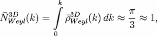
From an electrodynamic point of view, the central nontrivial aspect of Planck’s problem is that the average spectrum of the blackbody can be observed to be independent of the cavity shape. The explanation of this universality rests on the average spectral density of cavity modes, which is found to be independent of the resonator geometry to leading order in frequency. Although it may be intuitively convincing that the shape of the enclosure should become unimportant when its dimensions are large compared to the wavelength [81], the actual proof requires a large measure of ingenuity. In a series of works beginning in 1913 [82], Weyl showed that for a closed, three-dimensional electromagnetic resonator of volume V , the average spectral density as a function of wavenumber k is (including polarization)
 | (28) |
k then is  Weyl(k) Δk for large k. Geometric features other than the volume
enter in this quantity only as corrections with lower powers of the wavenumber. These terms
depend on the boundary conditions, surface area (or circumference) and curvature, as well as
on the topology of the cavity [83, 84].
As mentioned in the previous section, Eq. (26), microcavities can lead to enhanced
spontaneous emission because of their highly peaked density of electromagnetic modes.
Although Weyl’s formula is strictly valid only for short wavelengths, it nevertheless allows us
to estimate the limiting size for ultrasmall cavities that should be approached if we want to
observe such density-of-states effects: note that Eq. (28) approaches a “quantum limit” as the
volume V approaches (/2)3 at fixed wavelength : the number of modes with wavenumber
below k = 2
Weyl(k) Δk for large k. Geometric features other than the volume
enter in this quantity only as corrections with lower powers of the wavenumber. These terms
depend on the boundary conditions, surface area (or circumference) and curvature, as well as
on the topology of the cavity [83, 84].
As mentioned in the previous section, Eq. (26), microcavities can lead to enhanced
spontaneous emission because of their highly peaked density of electromagnetic modes.
Although Weyl’s formula is strictly valid only for short wavelengths, it nevertheless allows us
to estimate the limiting size for ultrasmall cavities that should be approached if we want to
observe such density-of-states effects: note that Eq. (28) approaches a “quantum limit” as the
volume V approaches (/2)3 at fixed wavelength : the number of modes with wavenumber
below k = 2 / is then
 | (29) |
Stability is a property of particular rays, not of a cavity as a whole. To understand all the
modes of a generic cavity, one has to go beyond paraxiality. It also must be realized that
paraxial optics is itself a special case of a more general approximation scheme, known as the
parabolic-equation method [85, 87]. This name refers to the fact that the resulting wave
equation of Schrödinger type is mathematically classified as a parabolic differential
equation. This is mentioned here because at a more abstract level, one can build
approximations of paraxial type not only around rectilinear rays: e.g., for WGMs, an envelope
function ansatz in polar coordinates, Ψ(r, φ) =χ (r;φ ) exp(-iβφ) allows to become the
“propagation direction”. The question of whether a mode can be called paraxial or
not then becomes dependent on the coordinate system one uses (e.g., Cartesian
vs. cylindrical). A more fundamental distinction by which the cavity as a whole
can be classified is that of integrability. Next, we discuss some examples for this
concept.
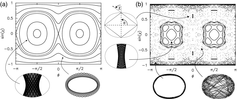
One feature that can be observed in both Fig. 2 (a) and (b) is that the modes exhibit caustics inside the dielectric, i.e. well-defined curves of high intensity which in the ray picture correspond to envelopes at which the rays are tangent. In the WGM, the caustic is an ellipse confocal with the boundary; it can be parameterized by its eccentricity, ec. In Fig. 2 (b), the caustic consists of two confocal hyperbola segments. Caustics separate the classically allowed from the forbidden regions, in the sense of the WKB approximation. In this section, we discuss some examples of how quasiclassical and exact solutions can be obtained in non-chaotic but nontrivial cavities, if coupling to the exterior region is neglected. In this closed limit, all fields can be written as real-valued functions obeying standard boundary conditions (Dirichlet or Neumann).
|
|
1,2(r) appearing in the quasiclassical ansatz for the wave,
![y(r) = A1(r) exp[- ik P1(r)] + A2(r) exp[- ikP2(r)]](acad2conv46x.gif) | (30) |
t). At least two terms are
necessary when there are two degrees of freedom; additional, symmetry-related terms may be
needed to make the wave field real-valued. In the standard EBK quantization, the amplitude
functions A1,2 are assumed to be slowly varying, and one can achieve the single-valuedness of
the wave function only if the phase advance in the exponentials is an integer multiple of 2 for
any closed loop in the planar cavity. This occurs only for certain discrete combinations
of the unknown parameters k (the wavenumber), and ec (the eccentricity of the
caustic). Hence, the semiclassical method quantizes not only the wave parameter k
of the modes, but also the classical parameter ec defining the corresponding ray
trajectories.
A simple example is the circular resonator, a limiting case of Fig. 3 (a). The internal
caustic in that case is a concentric circle with radius Ri. By geometry, the rays corresponding
to that caustic have a fixed angle of incidence given by sin = Ri/R, if R is the cavity radius.
Single-valuedness of the wave field then requires that the phase advance along a loop
encircling the caustic (= circumference × wavenumber) equals 2 m, where m is an integer:
 | (31) |
 nk as the linear
photon momentum, and recall the definition of classical angular momentum, L = r ×p. Then
if r lies on the surface, the z component of L is Lz = Rp sin , which identifies Lz = m by
comparing with Eq. (31). One can thus call m an “angular momentum quantum number”. In
addition to this orbital angular momentum quantization, there is a radial single-valuedness
condition which forces k to become discrete. This yields a complete set of two quantum
numbers for two degrees of freedom, and it implies that in Eq. (31) becomes discretized as
well – another way of understanding the quantization of the caustic ec. For a basic
discussion of the EBK method in rotationally invariant, separable cavity geometries,
cf. Ref. [89].
One result of the EBK quantization is that the WGMs do not in general correspond to
closed ray orbits except in the limit when the internal caustic approaches the cavity surface.
The quantized caustics instead belong to a family of rays which encircle the perimeter
quasi-periodically, coming arbitrarily close to any given point on the boundary after a
sufficiently long path length. This generalizes to most other resonator problems:
What counts for the formation of modes is not that the associated rays close on
themselves, but only that the wave fronts, to which these rays are normal, interfere
constructively.
nk as the linear
photon momentum, and recall the definition of classical angular momentum, L = r ×p. Then
if r lies on the surface, the z component of L is Lz = Rp sin , which identifies Lz = m by
comparing with Eq. (31). One can thus call m an “angular momentum quantum number”. In
addition to this orbital angular momentum quantization, there is a radial single-valuedness
condition which forces k to become discrete. This yields a complete set of two quantum
numbers for two degrees of freedom, and it implies that in Eq. (31) becomes discretized as
well – another way of understanding the quantization of the caustic ec. For a basic
discussion of the EBK method in rotationally invariant, separable cavity geometries,
cf. Ref. [89].
One result of the EBK quantization is that the WGMs do not in general correspond to
closed ray orbits except in the limit when the internal caustic approaches the cavity surface.
The quantized caustics instead belong to a family of rays which encircle the perimeter
quasi-periodically, coming arbitrarily close to any given point on the boundary after a
sufficiently long path length. This generalizes to most other resonator problems:
What counts for the formation of modes is not that the associated rays close on
themselves, but only that the wave fronts, to which these rays are normal, interfere
constructively.
Even in three-dimensional integrable cavities, the EBK method can yield highly accurate results down to the lowest-frequency modes. As an example, we mention recent work on a microlaser cavity with strong internal focusing properties, which consists of a dome in the shape of a paraboloid, on top of a layered semiconductor [90], cf. Fig. 3 (b). As in the ellipse, the exact solution for the mode shown for this plano-parabolic mirror geometry bears some resemblance to the more familiar paraxial optics, in this case a Gauss-Laguerre beam. However, just like the circular resonator, the parabolic dome has no stable ray orbits, owing to the confocal condition. The modes can be found exactly because the geometry allows separation of variables in parabolic cylinder coordinates.
The short-wavelength approximation can be made highly accurate (as in the parabolic dome) or even exact (as in the Fabry-Perot cavity of section 4). As a nontrivial generalization of exact quantization based on rays, Fig. 3 (c) shows the equilateral triangle. All its modes can be obtained by superimposing a finite number of suitably chosen plane waves [10, 91, 85]. This is achieved by “unfolding” the cavity into an infinite lattice created by its mirror images. These examples show that ray optics, as the skeleton which carries the wave fields, remains a useful tool far beyond the paraxial limit.
However, the reader may ask: what is the use for semiclassical methods in exactly solvable problems such as the above systems? After all, semiclassics is simple in separable systems! Beyond quantitative estimates, the value of quasiclassics is that the connection between modes and rays can be carried over to deformations of the cavity shape where the separability is destroyed. When this happens, eigenstates cannot be labeled uniquely by global quantum numbers anymore. However, as Weyl’s formula teaches us, the absence of good quantum numbers does not imply the absence of good modes. In order to classify the latter, we shall attempt to label them according to the ray trajectories to which they quasiclassically correspond.
|
|
 , the quadrupole is not an
integrable cavity and displays a far more intricate internal mode structure. In particular,
caustics become frayed, and nodal lines form ever more complicated patterns as
increases.
, the quadrupole is not an
integrable cavity and displays a far more intricate internal mode structure. In particular,
caustics become frayed, and nodal lines form ever more complicated patterns as
increases.
Given this complicated scenario, it is not immediately clear that ray considerations can help at all in understanding the properties of states such as those in Fig. 4. However, it turns out that quite the opposite is true: it is the added complexity of the internal ray dynamics that can be identified as the cause of the more complex wave fields. We make this somewhat provocative statement because the previous examples have proven the success of using ray considerations as a scaffolding for constructing the cavity modes. Unfortunately, there is so far no complete theoretical framework for the quasiclassical quantization of partially chaotic systems; the EBK method, which in quantum mechanics gives rise to the corrected Bohr-Sommerfeld quantization rules [88], fails when the system does not exhibit well-defined caustics, as was already noted by Einstein [92].
However, it is worth following the quasiclassical route because there exists a vast amount of knowledge about the classical part of the problem: chaotic ray dynamics can help gain insights into the wave solutions that cannot be gleaned from numerical computations alone. Ray optics can be formally mapped onto the classical mechanics of a point particle; this allows us to leverage a rich body of work on chaotic classical mechanics – a mature, though by no means complete field [1, 5, 93, 94]. Hence, quasiclassics in the presence of chaos is a challenging undertaking, but also a useful one because the numerical costs for obtaining exact wave solutions in nonintegrable systems are so high.
As observed in section 7, pulses that excite many cavity modes can behave ballistically, i.e. seem to follow well-defined trajectories. The idea of the quasiclassical approach is complementary to this: from the behavior of whole families of ray trajectories, we want to extract the properties of individual cavity modes.
As the ellipse already taught us, different types of ray motion can coexist in a single resonator
– e.g., WG and bouncing-ball trajectories. In such cases, it is desirable to know what
combination of initial conditions for a ray will result in which type of motion. Initial
conditions can be specified by giving the position on the boundary at which a ray is launched,
and the angle it forms with the surface normal. The proper choice of initial conditions was
identified at the end of section 4 as a prerequisite in the quasi-classical modeling of
resonance decay. The present section introduces the tools necessary for solving this
problem.
|
|
- sin plane, spanning all possible angles of incidence and
reflection positions along the boundary. The definition of in the center of Fig. 5 includes a
sign, measured positive in the direction shown by the arrow from the outward normal. This
reflects the observation made below Eq. (31) that sin is proportional to the z component of
the instantaneous angular momentum at the reflection, and the sign thus distinguishes the
sense of rotation.
By combining the two variables and sin , dynamical structure can be revealed which
would remain hidden in a collection of real-space ray traces. Non-chaotic trajectories are
confined by local or global conservation laws to one-dimensional lines, called invariant curves.
Almost all rays in the ellipse follow such curves, as seen in Fig. 5 (a), which shows a clearcut
division into oscillatory and rotational (WG) motion, cf. also Fig. 2. This is analogous to the
phase space of a physical pendulum [95]. The separatrix between the two types of
motion corresponds to a diametral ray orbit connecting the points φ= 0, π on the
boundary.
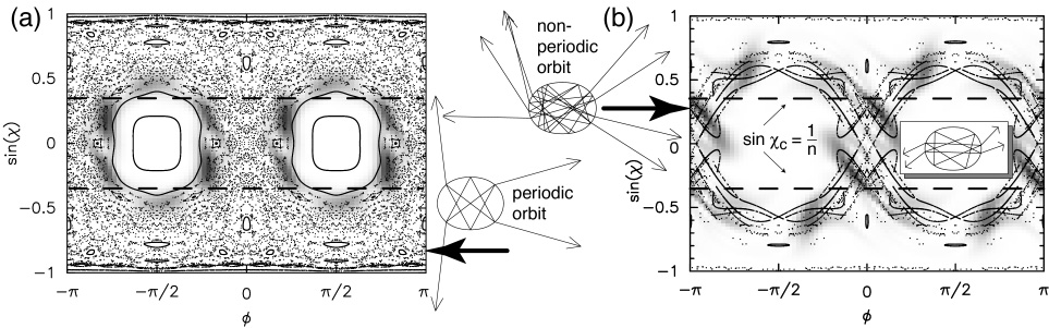
Rays launched on an invariant curve must remain on it for all subsequent reflections. Such
unbroken curves persist for | sin | 1 even in Fig. 5 (b); this is just the WG limit.
A lesser degree of robustness is observed for the oscillatory trajectories: they are
surrounded by elliptical “stable islands”, but a chaotic sea forms in-between, owing
to the fact that in Fig. 5 (b) the diametral separatrix orbit mentioned above is
unstable, developing the sensitivity to small deviations in initial conditions which is
typical for chaotic behavior. Chaos develops preferentially around such separatrix
orbits. The analogy to a pendulum makes this plausible: there, the separatrix is
the unstable equilibrium point at which the pendulum balances upside down. Note
that the different types of motion described here are mutually exclusive, i.e. chaotic
orbits never cross over into the islands of stability. This has the important effect
that chaotic motion is indirectly affected by the presence of stable structure in the
SOS.
The central reason why the SOS is introduced in this chapter is that it allows us to form a
bridge between the discrete electromagnetic modes of the cavity and their measurable emission
characteristics. Emission means coupling to the environment and hence appears as a
dissipation mechanism in the internal cavity dynamics, as illustrated in Eq. (9). Recalling
section 2, the emission from a dielectric cavity is governed foremost by Fresnel’s formulas,
which give a wavelength-independent relation for the reflectivities r along any ray path,
determined only by the local angle of incidence at reflection ; in the example of the
Fabry-Perot cavity, nothing else is needed to determine the decay rate of a cavity mode,
cf. Eq. (8). Now we note that the SOS shows the angle of incidence on the vertical axis, and
hence the Fresnel coefficient of any given reflection can be read off with ease. In
particular, the critical angle for TIR, Eq. (1), is represented in the SOS as a horizontal
line. When this line is crossed from above (in absolute value), refractive escape
becomes possible. The SOS then tells us which combinations of initial conditions give
rise to ray trajectories that eventually reach this classical escape window in phase
space.
To complete the bridge between a cavity mode and its corresponding set of initial
conditions in the ray dynamics, we have to find a way of projecting quasibound fields
onto the SOS. To this end, let us briefly discuss some aspects of how mode fields
can be measured. Individual quasibound states can be studied in great detail in
microlaser experiments [96, 97, 16, 98], because one can make spatially and spectrally
resolved images of the emitter under various observation angles. As is evident from
Fig. 4, the far-field intensity depends on the polar angle of the detector relative
to some fixed cross-sectional axis of the object (say, the horizontal axis). Instead
of simply measuring this far-field intensity, however, one can also ask from which
points on the cavity surface the collected light originated – i.e., an image of the
emitter can be recreated with the help of a lens. The dielectric will then exhibit
bright spots at surface locations whose distribution in the image may change as a
function of observation angle . The two variables and are conjugate to each other,
because measures a propagation direction whereas is a position coordinate of the
cavity.
The conjugacy between and means that they are incompatible, in the sense that they
obey an uncertainty relation: the field distribution as a function of in the image can be
deduced from the far-field distribution in by a Fourier transformation, and that is the
function performed by the imaging lens. But quantities related by Fourier transformation
cannot simultaneously have arbitrarily sharp distributions. Physically, in an image-field
measurement a large lens is needed to get good spatial () resolution, but this leaves a
larger uncertainty about the direction in which the collected light was traveling
[98].
If we could plot the measured intensity as a function of both and , we could generate a
two-dimensional distribution similar to the SOS of the preceding ray analysis. In fact, knowing
the surface shape, it is only a matter of trigonometry and the law of refraction to
transform the pair (, ) measured on the outside to (, ) inside the cavity and
hence make the analogy complete. But if one has already calculated the wave field of
a quasibound state, what is the advantage of representing it in this phase space
rather than in real space? The answer is that the real-space wave patterns often
obscure information about the correlations between the two conjugate variables
(, sin ). As mentioned above, the SOS which plots these variables would allow us to
understand whether a given mode is allowed to emit refractively; and if so, we can
furthermore determine at what positions on the surface and in which directions
the escape will preferentially occur. This is determined by the joint distribution of
(, sin ) over all reflections encountered by the rays corresponding to the given mode
[51].
To begin a phase space analysis, we now return to the question of how to extract correlations between conjugate variables from a wave field. This can be illustrated by analogy with a musical score: any piece of music can be recorded by graphing the sound amplitude as a function of time. On the other hand, musical notation instead plots a sequence of sounds by simultaneously specifying their pitch and duration. These are conjugate variables because monochromatic sounds require infinite duration [99], but their joint distribution is what makes the melody. The reason why musical scores can be written unambiguously is that they apply to a short-wavelength regime in which the frequency smearing by finite “pulse” duration goes to zero (in this sense, all music is “classical”. . . ). In the same way that musical notes are adapted to our perception of music, phase-space representations of optical wave fields project complex spatial patterns onto classical variables relevant in measurements.
This reasoning is familiar from quantum optics as well: there, amplitude and phase of the
electromagnetic field are conjugate variables, and their joint distribution is probed in
correlation experiments [100, 101]. A possible way of obtaining a phase-space representation is
the Husimi function, obtained by forming an overlap integral between the relevant quantum
state and a coherent state corresponding to a minimum-uncertainty wavepacket in the
space of photon number versus phase. Here, we want to extract the same type of
information about the joint distribution of the conjugate variables , sin relevant to an
optical imaging measurement on a cavity mode, as described above. By projecting
the electromagnetic field onto the SOS, measurable correlations are revealed which
can be compared to the classical phase space structure. This is another realization
of a Husimi function; the examples mentioned above differ essentially only in the
actual definition of the coherent state basis onto which the wave field is projected
[102].
Motivated by the above remarks on measurement of emission locations versus detector direction, we now note that the coherent states with which the cavity modes should be overlapped are in fact the Gaussian beams [2]. The fundamental Gaussian beam ψG has the property of being a minimum-uncertainty wavepacket in the coordinate x transverse to its propagation direction z, evolving according to the paraxial (Fresnel) approximation in complete analogy with a Schrödinger wavepacket,
![[ 2 ]
y (x,z) = ---1--- V~ --1-----exp - -----x------ exp(ikz).
G (2p)1/4 -iz 4s2 + 2iz/k
s + 2ks](acad2conv50x.gif) | (32) |
, and the angular beam spread is
 | (33) |
determines the spatial resolution. Only beams with angular spread
smaller than a maximum are admitted by the aperture, and hence features smaller than
the corresponding are unresolved. Clearly, the uncertainty product vanishes for high
wavenumbers.
We are concerned with the internal cavity, and thus do not want the definition to contain
the particular leakage mechanism (e.g., the law of refraction). Therefore, imagine
that our detector could be placed inside the cavity, close to its boundary. Given
the internal field ψint of the mode, we then make a hypothetical measurement by
forming the overlap with a minimum-uncertainty wavepacket ψG of width , centered
around a certain value of and sin . The form of ψG is analogous to Eq. (32), but
transformed to polar coordinates because our position variable is an angle, . The radial
coordinate can be eliminated because we constrained our detector to lie on the cavity
surface.
Although individual Gaussian wavepackets are not good solutions of the wave problem inside the cavity, they are always an allowed (though overcomplete) basis in which the field can be expanded. This is all we require in order to obtain the desired, smoothed phase space representation of ψint: The value of the overlap integral,
 | (34) |
and sin can (with some caveats) be interpreted as a phase space density,
and is the desired Husimi projection; the parameter in Eq. (32) should be chosen so as to
optimize the desired resolution in and sin , i.e., the “squeezing” of the minimum-uncertainty
wavepackets which probe ψint. Details on the definition, properties and applications of Husimi
functions on the ray phase space are found in Refs. [8, 103, 104, 105, 107, 97]. The price we
pay for obtaining a quasi-probability distribution is that Eq. (34) discards all phase
information.
Figure 6 shows how the prescription Eq. (34) maps the mode of Fig. 4 (c) and (d) onto
the classical ray dynamics. Although the chaotic trajectories corresponding to (d) show some
accumulation near certain paths in real space, only the Husimi plot reveals what
combinations of and sin occur in the internal field. This in turn determines at what
positions refractive ray escape is expected, and in which directions the light will radiate.
|
|
In this section, we return to the “mystery of the missing modes” with which section 8
confronted us: Weyl’s density of states is asymptotically the same for all cavities of the
same volume, even if we cannot classify their modes according some numbering that
follows from integrability, or at least paraxiality. Figure 4 shows that a given mode
does not cease to exist as integrability is destroyed with increasing , but evolves
smoothly into a new and complex field pattern with a well-defined spectral peak that
can even become narrower with increasing chaos in the ray dynamics. As noted in
section 10, the “mystery” is how at large shape deformation the increasingly numerous
chaotic rays, which crisscross the cavity in a pseudo-random way and even diverge
from each other, can give rise to constructive interference, and hence to a resonant
mode.
In section 9, the quasiclassical quantization approach led from the ray picture to the wave fields. Now, we follow the opposite direction and use the Husimi projection of a given cavity mode to perform a “dequantization” which leads to the ray picture. In this way, the novel physics of chaotic modes can be described without much technical detail.
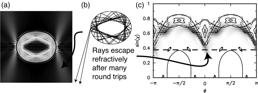
By superimposing the Husimi projection of a mode onto the SOS for the same deformation, we can identify classical structures on which the mode is built. We have so far encountered two types of structure, cf. the caption of Fig. 5: (I) invariant curves such as those formed by WG rays, permitting EBK quantization as discussed in section 9; (II) stable islands around periodic orbits, for which the paraxial approximation of the previous chapter [86] can be used. In both cases, a finite (and usually small) number of wavefronts suffices to achieve the constructive interference without which no cavity mode can form. The mode shown in Fig. 6, on the other hand, overlaps with neither of these non-chaotic phase-space components; it is a chaotic mode. One possible way to understand that chaotic modes are possible at all, is to realize that even the chaotic sea is not structureless.
The classical objects of crucial importance for an understanding of chaotic modes are the unstable periodic orbits of the cavity. They give rise to a third type of invariant sets in the ray dynamics: (III) stable and unstable manifolds. These are one-dimensional curves which, like the structures (I) and (II), have the property that rays launched anywhere on the manifold will always remain there. Along these manifolds, trajectories rapidly approach or depart from a given periodic orbit, such as the one shown in Fig. 6 (b, right inset). A non-periodic ray trajectory which moves along one of the corresponding manifolds is displayed in the top center inset.
The stable and unstable manifolds form an intricate web, the “homoclinic tangle”, which was already recognized by Poincaré as the cause of severe difficulties in calculating the dynamics [5]. Part of this tangle is shown in Fig. 6 (b), forming interweaving lobes which play an important role in controlling the transport of phase-space density. A discussion of this “turnstile” action and the relation to the stability of the orbits from which the tangle originates is found, e.g., in Refs. [1, 108]). As the Husimi projection in Fig. 6 (b) shows, the wave intensity is guided along the invariant manifolds of the unstable periodic orbit [110], imparting a high degree of anisotropy onto the internal intensity and on the emission directions.
Particularly strong Husimi intensity is found at the reflection points of the periodic orbit shown in the inset to Fig. 6 (b); this corresponds to the high-intensity ridges in the real-space intensity of Fig. 4 (d). Such wavefunction scarring [109] is a surprising feature, because a wave field concentrated near the origin of the homoclinic tangle, i.e., at the unstable periodic orbit itself, spatially appears similar to a sequence of Gaussian beams, despite the fact that paraxial optics requires the underlying modes to be stable. Even if we do not start from this paraxial point of view, but follow the historical developments in quantum chaos, scars seem to run counter to the early conventional wisdom that asserted chaotic modes should posses a random spatial distribution [108]. In a recent study on lasing in a large, planar laser cavity with no stable ray orbits [111], laser operation with focused emission was observed and explained by wave function scarring. This phenomenon is of interest not only from the applied point of view, but also because a complete understanding of the quasiclassical theory for modes corresponding to the invariant manifolds of type (III) is as yet missing [112, 113].
|
|
Chaotic WGMs are among the few types of chaotic modes for which an approximate quasiclassical description along the lines of section 9 is possible. They correspond to ray trajectories which are part of the chaotic sea but circulate along the cavity perimeter many times before exploring other phase-space regions, cf. Fig. 5 (b), bottom. There is thus a separation of time scales between the fast WG circulation and a slow deviation from WG behavior which inevitably ends in chaotic motion. This makes it possible to use an adiabatic approximation [114] in which the “diffusion” away from WG motion is neglected for times long enough to contain many round-trips of the ray.
As a consequence, one can formulate approximate quantization conditions for chaotic WG modes by ignoring the chaotic dynamics [51], leading to equations of the EBK type, Eq. (30). The approximate nature of this quantization can be recognized in Fig. 7 (a), which differs from the ellipse-shaped cavity of Fig. 2 (a) in the fact that a small but nonvanishing field persists in the cavity center. This indicates that there no longer is a well-defined caustic, as we required in section 9 Nevertheless, the Husimi distribution (grayscale) in Fig. 7 (c) condenses approximately onto a one-dimensional curve (the shape of which can be given analytically within the adiabatic approximation [51]), following the homoclinic tangle [the SOS in Fig. 7 (c) is vertically expanded compared to Fig. 6 (b)]. The location of this adiabatic invariant curve is determined by the EBK quantization; its minima are seen to approach the TIR condition.
As indicated in section 14, chaos does become important when the emission properties of a chaotic WG mode are concerned. It is the deviation of the rays from the above adiabatic assumption which allows an initially confined ray to violate the total-internal reflection condition after some time, and hence escape refractively, cf. Fig. 7 (b). In Fig. 7 (c), this escape results from wave intensity leaking across the TIR condition near φ= 0, π. This can be reproduced within a ray simulation by launching an ensemble of rays on the adiabatic invariant curve, and recording the distribution of classically escaping rays.
This implements the program outlined at the end of section 4 The stochastic branching of a ray trajectory into transmitted and reflected parts, also known as ray-splitting [48], could be summed up as a geometric series in the Fabry-Perot example, Eq. (6). In the oval cavity, Monte-Carlo simulations for large ensembles of incident rays are required [51]. This ray approach has been applied in scattering problems along the lines of Eq. (10) [49]; the value and applicability of ray considerations in scattering from chaotic optical cavities was demonstrated in Ref. [50]. The difference to the quasibound-state approach is that our incident rays are launched inside the cavity, not outside of it.
Because chaotic diffusion makes classical escape from WGMs possible in the first place, the
ray approach in fact becomes more useful at large deformations where chaos increases. That is
just the regime where exact scattering calculations encounter difficulties. Starting from the ray
approach to emission directionality and decay rates, one can then successively introduce
corrections at higher orders in . In particular, in Ref. [51], the openness of the system was
taken into account in the semiclassical quantization step by introducing additional phase shifts
into the EBK equations. The reason is that penetration into the outside region, as mentioned
in section 2, creates an enlarged, effective cavity boundary which lengthens the ray path
lengths. This “Goos-Haenchen effect” [15] is well-known from plane interfaces as
well. The effective cavity is actually of slightly different shape than the physical
geometry. This has the consequence that even the elliptic cavity of Fig. 2, which for
impenetrable boundaries is integrable, becomes non-integrable as a dielectric body
[46, 47].
In the 0 limit, the internal dynamics of the ellipse displays no chaos, cf. Fig. 5 (a). This
makes it an important test case with which to compare whenever we want to identify
fingerprints of chaos. The power of such comparisons has been illustrated in an experiment on
prolate, dye-doped lasing microdroplets [98]. The geometry of the droplets was rotationally
symmetric around the polar axis, which is also the major axis. If one analyzes only the light
propagating in a plane containing the two poles, then the cavity is effectively formed by the
2D axial cross section whose shape is an oval of the type we have been discussing above,
cf. Fig. 5. The experimental technique of recording with a CCD camera an image of the
micro-object at various observation angles (measured with respect to the polar axis of
a spheroidal droplet) reveals prominent bright and dark regions along the cavity
rim, from which the position and exit angle of the laser emission can be extracted
simultaneously.
As discussed in section 3, the lasing modes in low-index materials such as droplets should be of WG-type. The experiment illustrates both the focusing property, as well as the robustness of WGMs. When the lasing droplets are imaged from the side perpendicular to the polar axis (θ= 90o), one thus expects emission directionality of the type shown in Figs. 2 (a) or 7 (a), showing emission from the points of highest curvature (i.e., the poles). However, neither case describes the observed emission correctly. The droplets appeared dim at the poles instead of being brightest there.
This counter-intuitive phenomenon can be explained by the phase space structure shown in
Fig. 5 (b). An essential role is played by the small islands belonging to the stable
four-bounce diamond-shaped orbit depicted in the Figure. Its effect is that WG rays
of the type shown below the SOS are prevented from reaching the high-curvature
points (Φ= 0, π) at angle of incidence sinχ = 0.65, because chaotic and stable motion
are mutually exclusive (cf. section 11). Now TIR = arcsin 0.65 just happens to
be the critical angle for the droplet-air interface; hence, near-critical escape from
the highest-curvature points is ruled out for chaotically moving WG rays in the
droplet. In Fig. 5 (b), it is impossible to see from the ray trace in real space that the
combination φ= 0, χ=χ TIR will never occur. Likewise, this information is by no means
obvious from the wave equation itself Only the phase-space analysis using the SOS
reveals the small islands that cause this effect, which has been called dynamical
eclipsing. The emission profile is determined by the phase space structure in the vicinity
of the emission line sin TIR, and therefore we do not detect dynamical eclipsing
in the higher-index example of Fig. 7. A glance at Fig. 5 (a) makes it clear that
the effect will never occur in the ellipse, because the relevant islands do not exist
there.
The subtle difference in shapes between ellipsoid and quadrupole raises the question: How
short does the wavelength have to be compared to the cavity dimensions, in order to be able to
resolve such differences in geometry? Clearly, the droplets are so large compared to
the optical wavelength (35 m diameter for an equivalent-volume sphere) that we
are deep in the short-wavelength limit. What the above example teaches us is that
it is not the structure in real space that has to be resolved by the waves, but the
structure in phase space. The uncertainty principle will limit the size of the islands
that can have a noticeable effect on the cavity mode structure, but the important
thing to realize is that small differences in cavity shape can lead to large differences
in phase space structure. As a result, the phase space effects introduced in this
chapter turn out to be observable even in cavities that are not much larger than the
wavelength. This is an extension of the claim made for integrable systems in section
9, that quasiclassical methods often extend all the way to the longest-wavelength
modes.
Future work on nonintegrable dielectric cavities can proceed in various directions: our
understanding of the classical ray transport in partially chaotic systems has to be explored
further, and the systematic wave corrections to these ray ideas must be investigated.
Two such corrections which are of particular importance in chaotic systems are
dynamical localization [114, 51, 115] and chaos-assisted tunneling [107]. Dynamical
localization is an interference effect that suppresses decay rates below the value
expected from ray simulations as outlined in this chapter. It becomes more pronounced
in smaller cavities, and in fact helps maintain high Q-factors in the presence of
chaotic ray dynamics. Localization arises in many areas of physics as a name for wave
corrections to a classical diffusion picture. In our case, the diffusion happens in the
chaotic phase space of the ray dynamics. Chaos-assisted tunneling, on the other hand,
acts to enhance radiation losses of non-chaotic WGMs at small deformations when
chaos pervades only the low-sin regions of the SOS. It also leads to a coupling
between WG wavefronts encircling the cavity in counterclockwise and clockwise sense
of rotation, e.g., between the extreme bottom and top of the SOS in Fig. 4 (a).
In the ray picture, spontaneous reversal of rotation direction is forbidden for WG
trajectories on invariant curves; the mechanism at work here is tunneling in phase
space.
The phase space approach to microcavity electrodynamics provides a means of classifying the wide variety of modes in cavities where “good quantum numbers” do not uniquely enumerate the spectrum. Semiclassical methods provide the connection between individual modes and manifolds in phase space, such as the caustics in section 9, belonging to invariant curves in the SOS. Open questions remain about how to establish this connection in the general case when caustics are broken up by ray chaos. The particularly important case of WGMs, however, is amenable to approximate treatments which permit quantitative predictions. Many systems in which strong matter-field coupling enables quantum-electrodynamic studies, are actually large enough to be in the quasiclassical regime: examples are semiconductor domes [90] (where the effective wavelength is shortened by a high refractive index), or silica microspheres (cf. Ref. [21, 23] and citations therein) where atoms close to the dielectric interface interact evanescently with WGMs whose angular momentum according to Eq. (31) is m ~ 103. At all levels of microcavity optics – quantum or classical, linear or nonlinear – the fundamental task is to establish a modal basis, and the methods we sketched in this chapter accomplish this in a way that provides physical insight.
[1] Reichl, L. E. (1992). “The Transition to Chaos in Conservative Classical Systems: Quantum Manifestations,” Springer-Verlag, New York
[2] Siegman, A. E. (1986). “Lasers,” University Science Books, Mill Valley, CA
[3] Gutzwiller, M. C. (1998). Resource Letter ICQM-1: The interplay between classical and quantum mechanics. Am. J. Phys. 66, 304
[4] Heller, E. and Tomsovic, S. (1993). Post-modern quantum mechanics. Physics Today 46, 38.
[5] Gutzwiller, M. C. (1990). “Chaos in Classical and Quantum Mechanics,” Springer Verlag, New York.
[6] Child, M. S. (1991). “Quasiclassical Mechanics with Molecular Applications,” Clarendon Press, Oxford.
[7] Brack, M., and Bhaduri, R. K. (1997). “Quasiclassical Physics,” Frontiers in Physics 96, Addison-Wesley, Reading, USA.
[8] Smilansky, U. (1995). In: “Proc. 1994 Les Houches Summer School LXI on Mesoscopic Quantum Physics,” (E. Akkermans, G. Montambaux, J. L. Pichard and J.Zinn-Justin, Ed.) p. 373. Elsevier, Amsterdam.
[9] Stöckmann, H. J. (1999) “Quantum Chaos – an Introduction,” Cambridge University Press.
[10] Strutt, J. W., and Baron Rayleigh (1945). “The Theory of Sound,” Vol.II. Dover Publications, New York.
[11] Anderson, J. S., and Bratos-Anderson, M. (2000). Acoustic coupling effects in St. Paul’s Cathedral, London. J. Sound Vibr. 236, 209.
[12] Pipino, A. C. R. (1999). Ultrasensitive surface spectroscopy with a miniature optical resonator. Phys. Rev. Lett. 83, 3093.
[13] Johnson, B. R. (1993). Theory of morphology-dependent resonances: shape resonances and width formulas. J. Opt. Soc. Am. 10, 343.
[14] Nöckel, J. U., and Stone, A. D., In “ Optical Processes in Microcavities”, (R. K. Chang and A. J. Campillo, Eds.). World Scientific, Singapore.
[15] Snyder, A. W., and Love, J. D. (1991). “Optical Waveguide Theory,”. Chapman and Hall, London.
[16] Braun, I., et al. (2000). Hexagonal microlasers based on organic dyes in nanoporous crystals. Appl. Phys. B 70, 335.
[17] Kerker, M. (1969). “The Scattering of Light and Other Electromagnetic Radiation,” Academic Press, New York.
[18] v.d.Hulst, H. C. (1957). “Light scattering by small particles,” Wiley, New York.
[19] Nussenzveig, H. M. (1969). High-frequency scattering by a transparent sphere. I. Direct reflection and transmission. J. Math. Phys. 10, 82
[20] Barber, P. W. and Hill, S. C. (1990). “Light Scattering by Particles: Computational Methods,” World Scientific, Singapore.
[21] Sandoghdar, V., et al. (1996). Very-low threshold whispering-gallery microsphere laser. Phys. Rev. A 54, R1777.
[22] Vernooy,D. W., et al. (1998). Cavity QED with high-Q whispering-gallery modes. Phys. Rev. A 57, R2293.
[23] Kuritzki, G., et al. (2000). Control of atomic-state decay in cavities and microspheres. New J. Phys. 2, 1.
[24] Schmitt, C. G., and Arnott, W. P. (1999). Infrared emission (500-2000 cm-1) of laboratory ice clouds. J. Quant. Spectr. Rad. Trans. 63, 701
[25] Fields, M., Popp, J., and Chang, R. K. (2001). In “Progress in Optics,” (E. Wolf, Ed.), p.1. Elsevier Science Publishers.
[26] Yamamoto, Y., Slusher, R. E. (1993). Optical processes in microcavities. Physics Today 46, No. 6, 66.
[27] Chang, S. S. et al., (1999). Stimulated emission and lasing in whispering-gallery modes of GaN microdisk cavities. Appl. Phys. Lett. 75, 166.
[28] Nöckel, J. U. (2001). Optical feedback and the coupling problem in semiconductor microdisk lasers. submitted to physica status solidi.
[29] Roll, G., and Schweiger, G. (1998). Resonance shift of obliquely illuminated dielectric cylinders: geometric-optics estimates. Appl. Opt. 37, 5628.
[30] Poon, A. W., Chang, R. K., and Lock, J. A. (1998). Morphology-dependent resonances in an optical fiber: effects of fiber tilt and focused Gaussian beam illumination. Opt. Lett. 23, 1105.
[31] Artemyev, M. V., Woggon, U. and Wannemacher, R. (2001). Photons confined in hollow microspheres. Appl. Phys. Lett. 78, 1032.
[32] Mazumder, M. M., Hill, S. C., and P. W. Barber (1992). Morphology-dependent resonances in inhomogeneous spheres – comparison of the layered T-matrix method and the time-dependent perturbation method. J. Opt. Soc. Am. A 9, 1844; Chowdhury, D. Q., Hill, S. C., and Barber, P. W. (1991). Morphology-dependent resonances in radially inhomogeneous spheres, J. Opt. Soc. Am. A 8, 1702
[33] Chin, M. K., et al. (1999). GaAs microcavity channel-dropping filter based on a race-track resonator. IEEE Photon. Technol. Lett. 11, 1620.
[34] Benson, T. M., and Kendall, P. C. (1995). In “Methods for Modeling and Simulation of Guided-Wave Optoelectronic Devices: Part I, PIER 10,” (W. P. Huang, Ed.). EMW Publishing, Cambridge
[35] Lee, K. M., Leung, P. T., and Pang, K. M. (1998). Iterative perturbation scheme for morphology-dependent resonances in dielectric spheres. J. Opt. Soc. Am. A 15, 1383.
[36] Fan, X. D., et al. (2000). Coupling semiconductor nanocrystals to a fused-silica microsphere: a quantum-dot microcavity with extremely high Q-factors. Opt. Lett. 25, 1600.
[37] Waalkens, H., Wiersig, J., and Dullin, H. R. (1997). Elliptic quantum billiard. Ann. Phys. 260, 50
[38] Landau, L. D., and Lifshitz, E. M. (1979). “Quantenmechanik,” Akademie-Verlag Berlin.
[39] Lazutkin, V. F. (1993). “KAM Theory and quasiclassical Approximations to Eigenfunctions,” Springer, New York.
[40] Blatt, J. M., and Weisskopf, V. F. (1952). “Theoretical Nuclear Physics,” Wiley, New York.
[41] Xu, Y., Lee, R. K., and Yariv, A. (2000). Scattering-theory analysis of waveguide-resonator coupling. Phys. Rev. E 62, 7389.
[42] Taylor, J. R., (1972). “Scattering Theory,” Wiley, New York.
[43] Eckhardt, B. (1988). Irregular scattering. Physica D 33, 89.
[44] Blümel, R., and Smilansky, U. (1988). Classically irregular scattering and its quantum mechanical implications. Phys. Rev. Lett. 60, 477.
[45] Miller, W. H. (1975). In “Advances in Chemical Physics” 30, 77. (K. P. Lawley, Ed.) Wiley, New York.
[46] Yeh, C. (1963). Diffraction of waves by a penetrable ribbon. J. Math. Phys. 4, 65.
[47] Lock, J. A., et al. (1998). Amplification of high-order rainbows of a cylinder with an elliptical cross section. Appl. Opt. 37, 1527.
[48] Blümel, R., et al. (1996). Ray splitting and quantum chaos. Phys. Rev. A 53, 3284.
[49] Tränkle, E., and Riikonen, M. (2000). Elliptical halos, Bottlinger’s rings, and the ice-plate snow-star transition. Appl. Opt. 35, 4871.
[50] Jensen, J. H. (1993). Chaotic scattering of light by a dielectric cylinder. J. Opt.Soc. Am. A 10, 1204.
[51] Nöckel, J. U., and Stone, A. D. (1997). Ray and wave chaos in asymmetric resonant cavities. Nature 385, 45
[52] Hentschel, M., and Nöckel, J. U. (2001). The sequential-reflection model in deformed dielectric cavities. to be published in Proceedings of the Colloquium of the Royal Netherlands Academy of Arts and Sciences.
[53] Lamb, W. E., Schleich, W. P., Scully, M. O., and Townes, C. H. (1999). Laser physics: quantum controversy in action. Rev. Mod. Phys. 71, S263
[54] Vaynsteyn, V. A. 1969). “Theory of Open Resonators and open Waveguides,” Golem Press, Boulder; especially chapter 64.
[55] Moiseyev, N. (1998). Quantum theory of resonances: calculating energies, widths and cross-sections by complex scaling. Phys. Rep. 302, 211.
[56] Smith, F. (1960). Lifetime matrix in collision theory. Phys. Rev. 118, 349.
[57] Fyodorov, J., and Sommers, H.-J. (1997). Statistics of resonance poles, phase shifts and time delays in quantum chaotic scattering: random matrix approach for systems with broken time-reversal invariance. J. Math. Phys. 38, 1918
[58] Thirring, W. (1979). “ Quantum Mechanics of Atoms and Molecules” 3. Springer, New York.
[59] Friedel, J. (1958). Metallic alloys. Nuovo Cim. Ser. 10 Suppl. 7,287.
[60] Krein, M. G. (1962). Perturbation determinants and formula for traces of unitary self-adjoint operators. Sov. Math.-Dokl. 3, 707.
[61] Loyd, P. (1967). Wave propagation through an assembly of spheres. II The density of single-particle eigenstates. Proc. Phys. Soc. 90, 207.
[62] Loyd, P., and Smith, P. V. (1972). Multiple scattering theory in condensed materials. Adv. Phys. 21, 69.
[63] Faulkner, J. S. (1977). Scattering theory and cluster calculations. J. Phys. C 10, 4661.
[64] Gaspard, P. 1993). In Proc. of the International School of Phys. “Enrico Fermi”, Course CXIX, Varena (G. Casati, I. Guarneri and U. Smilansky , Eds.). North Holland, Amsterdam.
[65] Wirzba, A., and Henseler, M. (1998). A direct link between the quantum-mechanical and semiclassical determination of scattering resonances. J. Phys. A: Math. Gen. 31, 2155.
[66] Purcell, E.M. (1946). Spontaneous emission probabilities at radio frequencies. Phys. Rev. 69, 681.
[67] Heinzen, D. J., et al. (1987). Enhanced and inhibited spontaneous emission by atoms in a confocal resonator. Phys. Rev. Lett. 58, 1320.
[68] Meschede, D., (1992). Radiating atoms in confined space – from spontaneous emission to microlasers. Phys. Rep. 211, 201.
[69] Matinaga, F. M., et al. (1993). Low-threshold operation of hemispherical microcavity single-quantum-well lasers at 4 K. Appl. Phys. Lett. 62, 443.
[70] Brorson, S. D., and Skovgaard, P. M. W. (1996). In “ Optical Processes in Microcavities,” (R. K. Chang and A. J. Campillo, Eds.) World Scientific, Singapore.
[71] Hulet, R. G., Hilfer, E. S., and Kleppner, D. (1985). Inhibited spontaneous emission by a Rydberg atom. Phys. Rev. Lett. 55, 2137.
[72] Yablonovic, E. (1987). Inhibited spontaneous emission in solid-state physics and electronics. Phys. Rev. Lett. 58, 2059.
[73] Dittes, F.-M., Harney, H. L., and Müller, A. (1992). Non-exponential decay of a one-channel system. Phys. Rev. A 45, 701.
[74] Wolf, J.-P., et al. (2001). Ballistic trajectories of optical wavepackets within microcavities. submitted to Opt. Lett.
[75] Mürtz, M., Frech, B., and Urban, W. (1999). High-resolution cavity leak-out
absorption spectroscopy in the 10 m region. Appl. Phys. B 68, 243.
[76] Zhang, J.-Z., Leach, D. H., and Chang, R. K. (1988). Photon lifetime within a droplets – temporal determination of elastic and stimulated Raman scattering. Opt. Lett. 13, 270.
[77] Friedrich, H. (1991). “Theoretical Atomic Physics,” Springer Verlag, Berlin.
[78] Haake, F. (1992). “Quantum Signatures of Chaos,” Springer, Berlin.
[79] Kohler, A., and Blümel, R. (1998). Weyl-formulas for quantum ray-splitting billiards. Ann. Phys. 267, 249.
[80] Balian, R., and Bloch, C. (1970). Distribution of eigenvalues for the wave equation in a finite domain. I. Three-dimensional problem with smooth boundary surface. Ann. Phys. 60, 401.
[81] Yariv, A. (1975). “Quantum Electronics,” John Wiley, New York.
[82] Weyl, H. (1968). “Gesammelte Abhandlungen,” Springer Verlag, Berlin.
[83] Kac, M. (1966). Can one hear the shape of a drum? Am. Math. Monthly 73, 1.
[84] Eckhardt, B. (1988). Quantum mechanics of classically non-integrable systems. Phys. Rep. 163, 205.
[85] Laeri, F., and Nöckel, J. U. (2001). In “Handbook of Advanced Electronic and Photonic Materials” (H. S. Nalwa, Ed.) Academic Press, San Diego.
[86] Siegman, A. E., previous chapter in this volume
[87] Babi , V. M., and Buldyrev, V. S. (1972). “Short-Wavelength Diffraction
Theory,” Springer-Verlag, Berlin.
, V. M., and Buldyrev, V. S. (1972). “Short-Wavelength Diffraction
Theory,” Springer-Verlag, Berlin.
[88] Keller, J. B., and Rubinow, S. I. (1960). Asymptotic solution of eigenvalue problems. Ann. Phys. 9, 24.
[89] Roll, G., and Schweiger, G. (2000). Geometrical optics model of Mie resonances. J. Opt. Soc. Am. A 16, 882.
[90] Nöckel, J. U., et al. (2000). Mode structure and ray dynamics of a parabolic-dome microcavity. Phys. Rev. E 62, 8677.
[91] Richens, P. J., and Berry, M. V. (1981). Pseudointegrable systems in classical and quantum mechanics. Physica 2D, 495.
[92] Einstein, A. (1917). Zum Quantensatz von Sommerfeld und Epstein. Verh. Deut. Phys. Ges.
[93] Arnol’d, V. I. (1989). “ Mathematical Methods of Classical Mechanics, “ Springer, New York.
[94] Zaslavsky, G. M. (1999). Chaotic dynamics and the origin of statistical laws. Physics Today 52 No. 8, 39.
[95] Goldstein, H. (1980). “Classical Mechanics,” 2nd ed. Addison-Wesley, Reading, MA.
[96] Mekis, A., et al. (1995). Ray chaos and Q-spoiling in lasing droplets. Phys. Rev. Lett. 75, 2682.
[97] Gmachl, C., et al. (1998). High power directional emission from lasers with chaotic resonators. Science 280, 1556.
[98] Chang, S. S., Nöckel, J. U., Chang, R. K., and Stone, A. D. (2000). Observation of emission from chaotic lasing modes in deformed microspheres: displacement by the stable orbit modes. J. Opt. Soc. Am. B 17, 1828.
[99] Bartelt, H. O., Brenner, K.-H., and Lohmann, A. W. (1980). The Wigner distribution function and its optical production. Opt. Commun. 32, 32.
[100] Walls, D. F., and Milburn, G. J. (1994). “Quantum Optics,” Springer, Berlin.
[101] Raymer, M. G., Beck, M., and McAlister, D. F. (1994). Complex wave-field reconstruction using phase-space tomography. Phys. Rev. Lett. 72, 1137.
[102] LeBoeuf, P., and Saraceno, M. (1990). Eigenfunctions of non-integrable systems in generalized phase-spaces. J. Phys. A: Math. Gen. 23, 1745.
[103] Crespi, B., Perez, G., and Chang, S.-J. (1993). Quantum Poincaré sections for two-dimensional billiards. Phys. Rev. E 47, 986.
[104] Tualle, J.-M., and Voros, A. (1995). Normal modes of billiards portraied in the stellar (or nodal) representation. Chaos, Solit. Fract. 5, 1085.
[105] Frischat, S. D., and Doron, E. (1997). Quantum phase-space structures in classically mixed systems: a scattering approach. J. Phys. A: Math. Gen. 30, 3613.
[106] Klakow, D., and Smilansky, U. (1996). Wave functions, expectation values and scars on Poincaré sections – a scattering approach. J. Phys. A: Math. Gen. 29, 3213.
[107] Hackenbroich, G., and Nöckel, J. U. (1997). Dynamical tunneling in optical cavities. Europhys. Lett. 39, 371.
[108] Bohigas, O., Tomsovic, S., and Ullmo, D. (1993). Manifestation of classical phase space structures in quantum mechanics. Phys. Rep. 223, 43, and references therein.
[109] Heller, E. (1984). Bound-state eigenfunctions of classically chaotic Hamiltonian systems: scars of periodic orbits. Phys. Rev. Lett. 53, 1515.
[110] Schweizer, W., Jans, W., and Uzer, T. (1998). Optimal localization of wavepackets on invariant structures. Phys. Rev. B. 58, 1382.
[111] Fukushima, T., et al., (1998). Beam-propagation behavior in a quasi-stadium laser diode. Optics Express 2, No. 2, p.21.
[112] Tomsovic, S., and Heller, E. (1993). Quasiclassical construction of chaotic eigenstates. Phys. Rev. Lett. 70, 1405.
[113] Kaplan, L. (1999). Scar and antiscar quantum effects in open quantum systems. Phys. Rev. E 59, 5325.
[114] Nöckel, J. U. (2001). Angular momentum localization in oval billiards. Physica Scripta T 90, 263.
[115] Starykh, O. A., et al. (2000). Signature of dynamical localization in the resonance width distribution of wave-chaotic dielectric cavities. Phys. Rev. E 62, 2078.

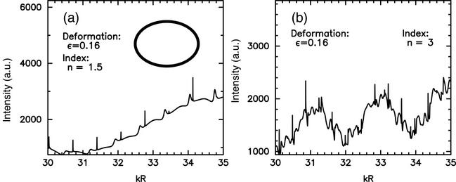
 . The length scale
  is used in our calculations to convert the
wavenumber into the dimensionless “size parameter”
is used in our calculations to convert the
wavenumber into the dimensionless “size parameter” 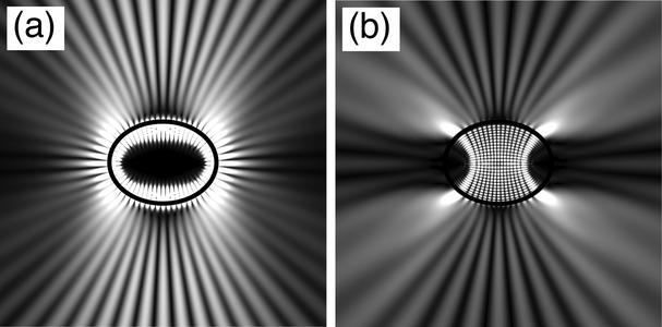
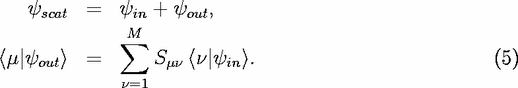
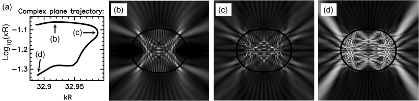

 . Here,