Progress in Cryogenic Fluid Mechanics

This informal report is an attempt to give an overall picture of research in fluid mechanics using low temperature techniques at the University of Oregon and Yale University over the past several years. This effort has been a prime example of the felicitous application of low temperature techniques to other fields. We first became interested in these possibilities in the late 1980’s when the (old) idea of a superfluid wind tunnel was seriously reexamined.

• Thermal convection

            Those  devoted to the study of quantum fluids are aware of the unprecedented  sorts of fluid dynamics that occur when superfluids are present.  What has been slow for many of us to grasp are the other extraordinary fluid mechanical  tools low temperature physics provides.  A prime example is in the field of thermal convection.  A layer of fluid of height L heated from below and cooled from above produces a temperature difference DT and an associated gradient in the density r. For typical fluids with a positive thermal expansion coefficient, the denser fluid lies above the less dense fluid, creating a gravitationally unstable configuration.  For small DT, the layer remains at rest.  But if  DT is large enough, convection will occur.  Just above the onset of convection, the flow takes the form of closed circular stream lines.  If the flow is visualized from above, the flow pattern consists of bands of up-and-down flows called convection rolls.  With further increases in DT, the rolls become unstable.  This typically results in unsteady or time dependent flow.  With yet further increase in DT, the time-dependence passes through a chaotic regime where the rolls are still identifiable, but where the motion is difficult to predict.  For even larger DT, the roll structure is lost, and turbulent flow sets in. 

There are several parameters which determine the character of the flow.  The key control parameter is the Rayleigh number, Ra, which is a dimensionless measure of DT. 

with

a  Isobaric thermal expansion coefficient

k  Thermal diffusivity

L  Height of the convecting layer

 Adverse temperature drop across the layer

g     Acceleration of gravity

The dynamical equations for Rayleigh-Bénard convection contain only Ra and the Prandtl number . In addition, the flow depends on the geometry of the container, as expressed by the aspect ratio G = D/L, where D is the diameter.  Thus, the scaled flow properties should be the same for two systems having the same set of parameters Ra, Pr and G (assuming that the geometry remains unaltered).  The structure of flows as a function of Ra is important for understanding the reasons for a large scale convective turbulence experiment.  The larger the Ra, the larger is the range of scales excited in the turbulent flow.  Ra can be made large by choosing the fluid such that the combination a/kn is large, by making DT large, or by making L large.  To our knowledge, low temperature helium is the optimum fluid by a substantial margin for making a/kn large.  The quantity a/kn can be a million times larger for helium gas near the critical point than for water.  Various choices for fluids of different kinematic viscosity are shown in the plot below.  Although, in principle, DT could be made large, this is undesirable because the fluid will then no longer obey the Boussinesq approximation, rendering the theory considerably more difficult.  For instance, for large DT, the density could no longer be assumed to depend linearly on temperature.  Because Ra depends on the third power of L, extremely large Rayleigh numbers can be attained by making L large. 

The heat flux, q, plays an obviously important role in Rayleigh-Bénard convection, since it generates the temperature difference, DT.  Note that q = Q/A where A is the cross-sectional area of the apparatus, and Q is the heat current.  It is convenient to define a dimensionless measure of the heat transport, the Nusselt number, Nu: Nu = Q/Q_c where Q_c is the portion of the heat current carried by conduction alone.  Note that Nu depends only on the dimensionless parameters of the problem, i.e. Ra, Pr and G.

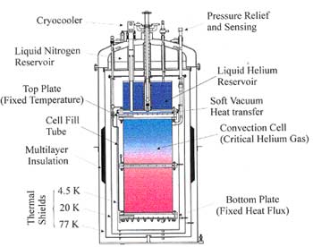
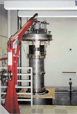
Brian Pippard realized before anyone else  the utility of critical helium gas, and his graduate student Threlfall was the first to show the great range of Rayleigh numbers possible in one apparatus, achieving Rayleigh numbers from 60 to 2x10⁹.  Threlfall’s work stimulated a great deal of theoretical and experimental work at Chicago under the leadership of Albert Libchaber and Leo Kadanoff.  Libchaber’s graduate student X. Wu managed to reach a Rayleigh number of 10¹⁴ in a larger cell than used by Threlfall. The difficulty with the aforementioned results is that they disagreed with the theoretically expected power law dependence .  After much turmoil, the theorists came forth with Nu~Ra ^2/7 which was somewhat near Wu’s results.

            When the SSC was terminated, DOE ran a competition to find uses for resources like liquid helium plants.  We competed successfully and were able to draw up conceptual designs for a 10 m high convection tank that  would, in principle, achieve Rayleigh numbers of 10²², ie. of interest in astrophysical fluid dynamics.  This is still in the future.  However with the help of NSF, we proceeded to  plan and construct a 1m high Bénard cell , and were able to reach Ra~10^17.  The apparatus and results are shown below. 

            To the best of our knowledge this figure represents the largest dynamical range observed (11 decades in Rayleigh number) in any single run in physics on one apparatus.¹

Quantum turbulence: an unexpected surprise

            For the past half century there have been hundreds of experiments reported from the United States and abroad on the phenomenon of counterflow turbulence.  Counterflow turbulence is the form of quantized vortex tangle in the superfluid component excited when a closed tube containing helium II, heated at one end and cooled at the other, is given a heat flux beyond some small critical value.  This flow has no classical analogue.  While these experiments are relatively easy to carry out, there are many aspects still poorly understood, such as the consequences of different aspect ratios and shapes of channel and such fundamental questions as to whether the normal fluid itself is turbulent or not.  The most important tool in this field of investigation was developed by Joe Vinen: namely the attenuation of second sound by the presence of quantized vortex lines, which give a measure of the RMS vorticity (curl) of the flow averaged over the channel.²

What has changed all this is the initiation of a new form of turbulent flow created by a grid towed through a sample of stationary helium II. The towing of the grid (typically in a 1x1cm² channel) provides a wide range of initial vorticities by simply towing at different speeds which can then be examined as the flow decays.³

The major surprise in these experiments was the unexpected classical behavior of the flow ^4.  Second sound sees only quantized vortex lines and just why they should mimic classical flows is a profound challenge. Evidently the quantized vortex lines tend to mimic the turbulence in the normal fluid.  A deep discussion of this has been given by Joe Vinen.^5.

The decay of turbulent quantized vorticity generated by a moving grid in superfluid helium is shown below. The close correspondence with the classical decay rate is both unmistakable and astounding. 

            One of the most surprising things to arise in the theory of quantum turbulence is the question of just how turbulence decays below 1 K when no normal fluid is present.  Viscosity does the job for ordinary fluids, but superfluid turbulence well below 1 K decays about the same as above 1 K.  This is the subject of an extended theoretical, simulation and  experimental investigation by Joe Vinen and colleagues in the UK and Japan.

Dissipation in Turbulent Helium II

            The dissipation per unit mass in a classical turbulent flow is of the form

where is the kinematic viscosity of the fluid and  is the mean square vorticity.  The question then for helium II is: what takes the place of  ?  One choice favored for many years is , where  is the viscosity and  the total density of helium II although the choice seems even more logical.  Thanks to the towed grid experiment’s similarity in decay to classical fluids, it is possible to deduce the actual value  of the effective kinematic viscosity of the two coupled fluids.  The results are shown below, and it is seen that  is a completely new quantity in quantum turbulence.⁶

Tow tanks and wind tunnels

            It has been known since the closing days of World War II that using low temperatures greatly improves the efficiency and ultimate Reynolds numbers of wind tunnels.  Cooling raises the density and lowers the viscosity of air, leading to lower kinematic viscosity and hence higher Reynolds numbers.

Early studies in our group showed that a wind tunnel using liquid helium as a test fluid could be used to test submarine models at full Reynolds number appropriate to a nuclear submarine at full throttle.⁸.  Tow tanks also have remarkable new possibilities ⁸. 

What we have come slowly to realize, however, is the tremendous flexibility in fluid properties offered by critical helium gas: something brought to our attention in the convection experiments discussed above.  We have constructed a recirculating critical helium gas tunnel shown below.  Our preliminary tests were at 6.5 K with mesh Reynolds numbers around 1500.  The grid generated turbulence was probed with the 10 micron diameter hot wire described below.  The hot wire obeyed King’s law relating velocity and voltage, and time series exhibited standard statistical features. One of the optimal operating points for high Re flow will be at 4 bar pressure and 6 K.  Mesh Reynolds numbers of 30,000 to 100,000 will be available, and the corresponding microscale Reynolds numbers will range from 150 to 280.  This first small step takes cryogenic wind tunnels down in temperature by more than a factor of 10 (from 77 K). The  tunnel is illustrated in the figure below. The black object is a computer box fan (suggested by Roger Arndt) and the fan is driven by a magnetic coupling from outside.

Pipeflow

            We have shown that an unusually small pipe flow apparatus using both liquid helium and room temperature gases can span an enormous range of Reynolds numbers.  This paper ⁹ describes the construction and operation of the apparatus in some detail.  A wide range of Reynolds numbers is an advantage in any experiment seeking to establish scaling laws. Using a flow pipe only 28 cm long and 0.4672 cm in diameter we were able to span a Reynolds number range from 10 to 10⁶ by taking advantage of the variation in the kinematic viscosity of the fluids used.  Recently Lex Smit’s group at Princeton University has used the (28 ton!) Superpipe to reach Reynolds number to 35 million using highly compressed air.  Combining their data and ours on one plot shows the largest range of friction factors for smooth pipe flow ever achieved.  The range of fluids and the accuracy of the data is a tribute to the power of dynamical similarity in fluid mechanics. This plot will likely replace the standard diagram appearing in almost every fluid mechanical text ever written.

Hot wire anemometers

Although helium I is a Navier-Stokes fluid, the possibility of generating ever higher Reynolds numbers carries with it ever decreasing Kolmogorov lengths. For example in a 10 cm pipe characteristic lengths at the highest Reynolds numbers could be less than 50 Angstroms.

Hot wire anemometers are resistive self-heating devices which balance heat lost to flow, which depends on the fluid velocity. Calibration provides the correlation between fluid velocity and electrical power supplied. Standard hot wires have a diameter of order 5µm and length ~1000µm. Standard materials (e.g. platinum) used at room temperature are insensitive at low temperature.

Our cryogenic hot wires anemometers are made on a quartz fiber of diameter 10 microns. They consist of an evaporated Au-Ge film of thickness of order 3000 Å. A small sensitive region in middle of the fiber is defined by masking the fiber and evaporating a metallic film over it. Masking is achieved by laying a small diameter fiber perpendicular to the first fiber. The metal film provides electrical contact to the sensitive region.


The figure below shows how the small sensors are mounted. Sensor support dimensions follow the “rule of 10”: they are placed ten times (more or less) their characteristic dimension away from the sensitive region. Electrical contact to the fiber is made through stainless steel wires, which are isolated from the brass ring by epoxy. The fiber is fastened to the wires using an electrically conducting epoxy.

PIV

            One of the most important goals we had was to find a was to implement Particle Image Velocimetry (PIV).  One reason is that this widely used technique in fluid mechanics would probably work in both helium I and helium II.  The simplest experiment we could think of was a variant on the towed grid apparatus described above.  A small cryostat purchased from Janis Dewars was retrofitted with a towed grid device as shown below.  The design and implementation of the cryogenics was done at Oregon and transferred to Yale.  There Christopher White  did a most interesting dissertation on implementing PIV in cooperation from Dr. Adonios Karpetis.  The details of this work are ably explained in White’s thesis, and demonstrate beyond doubt that PIV will work in liquid helium.¹⁰

References

(These are a few key papers.  Full bibliographical references are in our detailed papers.)

1. "Turbulent Convection at High Rayleigh Numbers", J. J. Niemela, L. Skrbek, K. R. Sreenivasan and R. J. Donnelly. Nature 404: 837-841 (2000).

2. "Mutual Friction in a Heat Current in Liquid Helium II, I. Experiments on Steady Heat Currents", W. F. Vinen. Proc. Roy. Soc. London(114-27)(1957).

3. "Decay of Vorticity in Homogemeous Turbulence", M. R. Smith, R. J. Donnelly, N. Goldenfeld and W. F. Vinen. Phys. Rev. Lett. 71: 2538-2586 (1993).

4. "Four Regimes of Decaying Turbulence in a Finite Channel", L. Skrbek, J. J. Niemela and R. J. Donnelly. Phys. Rev. Lett. 85: 2973-2976 (2000).

5. "Classical character of turbulence in a quantum fluid", W. F. Vinen. Physical Review B 61: 1410-1420 (2000).

6. "Dissipation of Grid Turbulence in Helium II", S. Stalp, J. J. Niemela, W. F. Vinen and R. J. Donnelly. Physics of Fluids 14: 1377-1379 (2002).

7."The Flow About a Torsionally Oscillating Sphere", R. Hollerbach, R. J. Wiener, I. S. Sullivan and R. J. Donnelly. Physics of Fluids 14: 4192-4205 (2002).

8 "Liquid and Gaseous Helium at Test Fluids", R. J. Donnelly in. High Reynolds Number Flows Using Liquid and Gaseous Helium R. J. Donnelly, Ed., New York, 1989. Springer-Verlag 284 (1991).

9. "Pipe Flow Measurements over a Wide Range of Reynolds Numbers Using Liquid Helium and Various Gases", C. J. Swanson, B. Julian, G. G. Ihas and R. J. Donnelly. J. Fluid. Mech. 461: 51-60 (2002).

10. “High Reynolds Number Turbulence in Small Apparatus”. C. M. White . PhD Thesis, Mechanical Engineering, Yale University: 112pp.(2001)