Basic Light Curve Fitting

To get an idea of building and interacting with the illumination posterior class, we’ll simulate an exoplanet and photometric observations, and fit the simulated data.

Simulate observations

First we need the modules:

import numpy as np
import healpy as hp

from scipy.optimize import minimize

from matplotlib import pyplot as plt

from exocartographer.gp_map import draw_map
from exocartographer import IlluminationMapPosterior
from exocartographer.util import logit, inv_logit

Now we’ll simulate an exoplanet to observe. We’ll define some properties of the Gaussian process (GP) describing the exoplanet, specifically the angular length scale of features on the planet surface (we’ll use 30 degrees), mean (0.5) and standard deviation (0.2) of the kernel, and the relative amplitude of the white noise on top of the GP:

sim_nside = 8  # map resolution

# Gaussian process properties
sim_wn_rel_amp = 0.02
sim_length_scale = 30. * np.pi/180
sim_albedo_mean = .5
sim_albedo_std = 0.25

# Draw a valid albedo map (i.e., 0 < albedo < 1)
while True:
    simulated_map = draw_map(sim_nside, sim_albedo_mean,
                             sim_albedo_std, sim_wn_rel_amp,
                             sim_length_scale)
    if min(simulated_map) > 0 and max(simulated_map) < 1:
        break

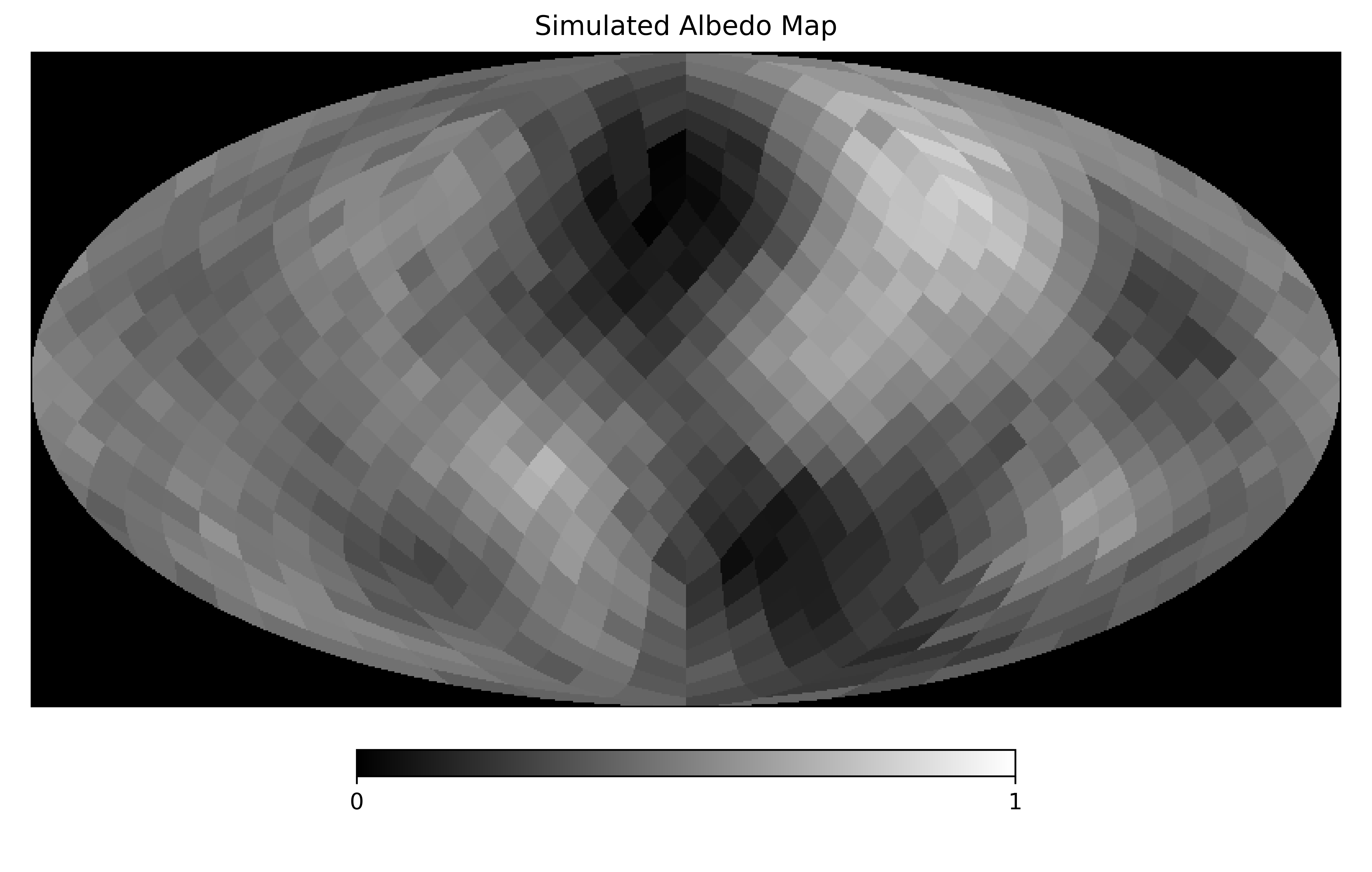
hp.mollview(simulated_map, min=0, max=1,
            title='Simulated Albedo Map', cmap='gist_gray')

Now we’ll define the orbital properties to simulate (Earth-like rotational and orbital periods, 90 degree inclination and obliquity), and the observation schedule (5 epochs, each with 24 hourly observations, spread over an orbital period):

# Set orbital properties
p_rotation = 23.934
p_orbit = 365.256363 * 24.0
phi_orb = np.pi
inclination = np.pi/2
obliquity = 90. * np.pi/180.0
phi_rot = np.pi

# Observation schedule
cadence = p_rotation/24.
nobs_per_epoch = 24
epoch_duration = nobs_per_epoch * cadence

epoch_starts = [30*p_rotation, 60*p_rotation, 150*p_rotation,
                210*p_rotation, 250*p_rotation]

times = np.array([])
for epoch_start in epoch_starts:
    epoch_times = np.linspace(epoch_start,
                              epoch_start + epoch_duration,
                              nobs_per_epoch)
    times = np.concatenate([times, epoch_times])

To generate the simulated observations we’ll make use of the IlluminationMapPosterior, fixing the orbital parameters and using the simulated map to generate the true light curve. To simulate actual observations we’ll add a normally distributed component with a fractional standard deviation of 0.001:

measurement_std = 0.001

truth = IlluminationMapPosterior(times, np.zeros_like(times),
                                 measurement_std, nside=sim_nside)

true_params = {
    'log_orbital_period':np.log(p_orbit),
    'log_rotation_period':np.log(p_rotation),
    'logit_cos_inc':logit(np.cos(inclination)),
    'logit_cos_obl':logit(np.cos(obliquity)),
    'logit_phi_orb':logit(phi_orb, low=0, high=2*np.pi),
    'logit_obl_orientation':logit(phi_rot, low=0, high=2*np.pi)}
truth.fix_params(true_params)
p = np.concatenate([np.zeros(truth.nparams), simulated_map])

true_lightcurve = truth.lightcurve(p)
obs_lightcurve = true_lightcurve.copy()
obs_lightcurve += truth.sigma_reflectance * np.random.randn(len(true_lightcurve))

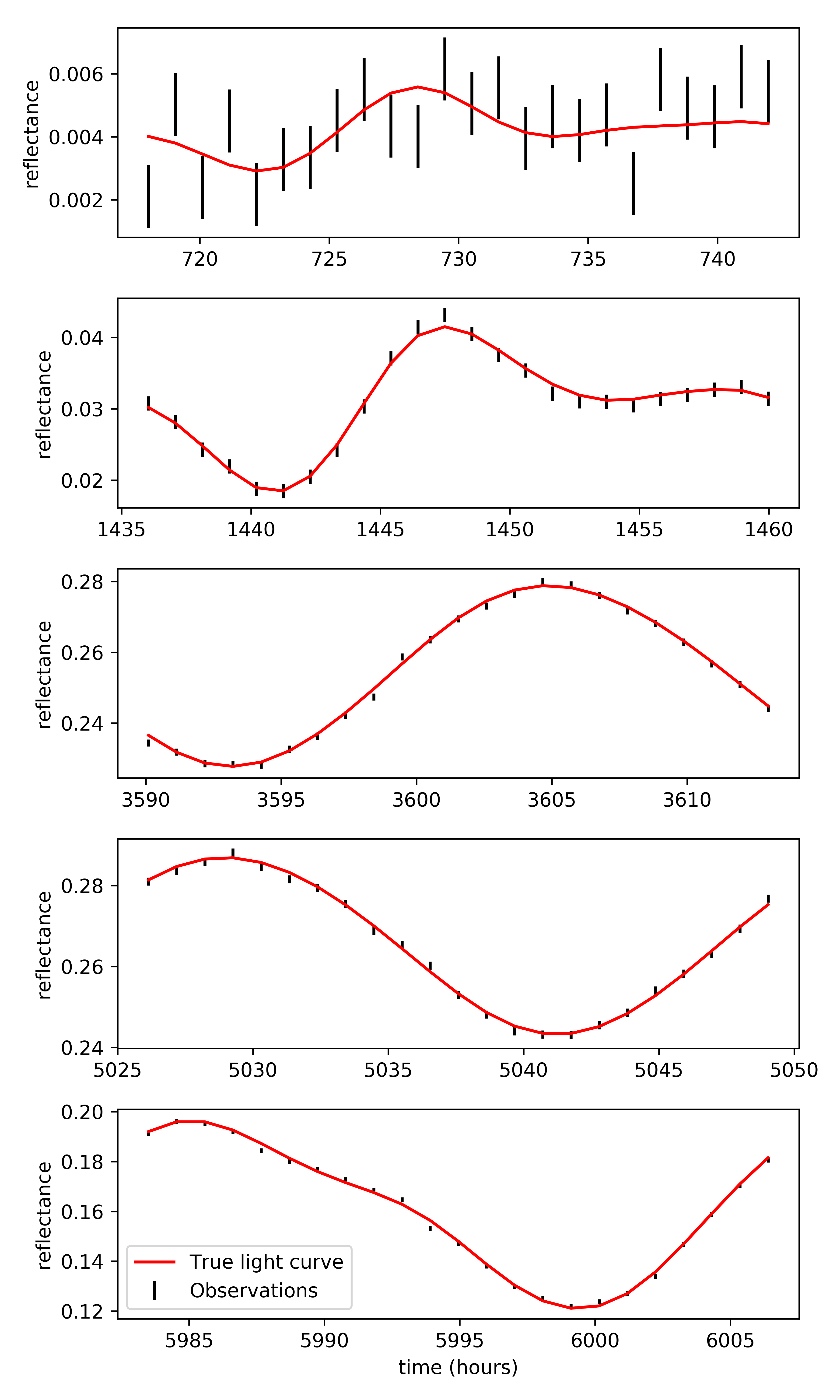
This is the data we have to fit:

fig, axs = plt.subplots(len(epoch_starts), 1,
                        figsize=(6, 2*len(epoch_starts)))

for ax, epoch_start in zip(axs, epoch_starts):
    sel = (times >= epoch_start) & \
            (times - epoch_start < epoch_duration)
    ax.plot(times[sel], true_lightcurve[sel],
            color='r', label='True light curve')
    ax.errorbar(times[sel], obs_lightcurve[sel],
                truth.sigma_reflectance[sel],
                capthick=0, fmt='o', markersize=0,
                color='k', label='Observations')

    ax.set_ylabel('reflectance')
axs[-1].set_xlabel('time (hours)')
axs[-1].legend(loc='lower left')

Fitting observations

With simulated observations in hand we can now try to fit the albedo map of the planet, where by “fit” we mean generate a point estimate for the albedo map parameters by maximizing the posterior probability density. To do this we’ll create an IlluminationMapPosterior instance with a resolution of \(N_\mathrm{side}=4\):

nside = 4
logpost = IlluminationMapPosterior(times, obs_lightcurve,
                                   measurement_std,
                                   nside=nside, nside_illum=4)

Here we set nside_illum=nside, which sets the resolution of the illumination kernel. Nature uses an infinite resolution for this, but that’s expensive to simulate. A high resolution here is ideal (e.g., 16); resolutions too low cause unphysical short-timescale variations in the light curve. We’re not looking for a rigorous fit here, so 4 should do.

We’ll just focus on fitting the map for now, so we’ll fix the orbital parameters to their simulated values. The posterior class by default doesn’t trust observers, and adds an extra parameter that scales the measurement uncertainties. For now we’ll trust our own uncertainties and fix this parameter to 1.:

fix = true_params.copy()
fix['log_error_scale'] = np.log(1.)

logpost.fix_params(fix)

Let’s pick some random starting values for the unfixed parameters:

p0 = np.random.randn(logpost.nparams)

mu0 = 0.5
sigma0 = .1
wn_amp0 = 0.05
scale0 = np.random.lognormal()

while True:
    map0 = draw_map(nside, mu0, sigma0, wn_amp0, scale0)
    if min(map0) > 0 and max(map0) < 1:
        break

pnames = logpost.dtype.names
p0[pnames.index('mu')] = mu0
p0[pnames.index('log_sigma')] = np.log(sigma0)
p0[pnames.index('logit_wn_rel_amp')] = logit(wn_amp0,
                                             logpost.wn_low,
                                             logpost.wn_high)
p0[pnames.index('logit_spatial_scale')] = logit(scale0,
                                                logpost.spatial_scale_low,
                                                logpost.spatial_scale_high)

p0 = np.concatenate([p0, map0])
print("log(posterior): {}".format(logpost(p0)))

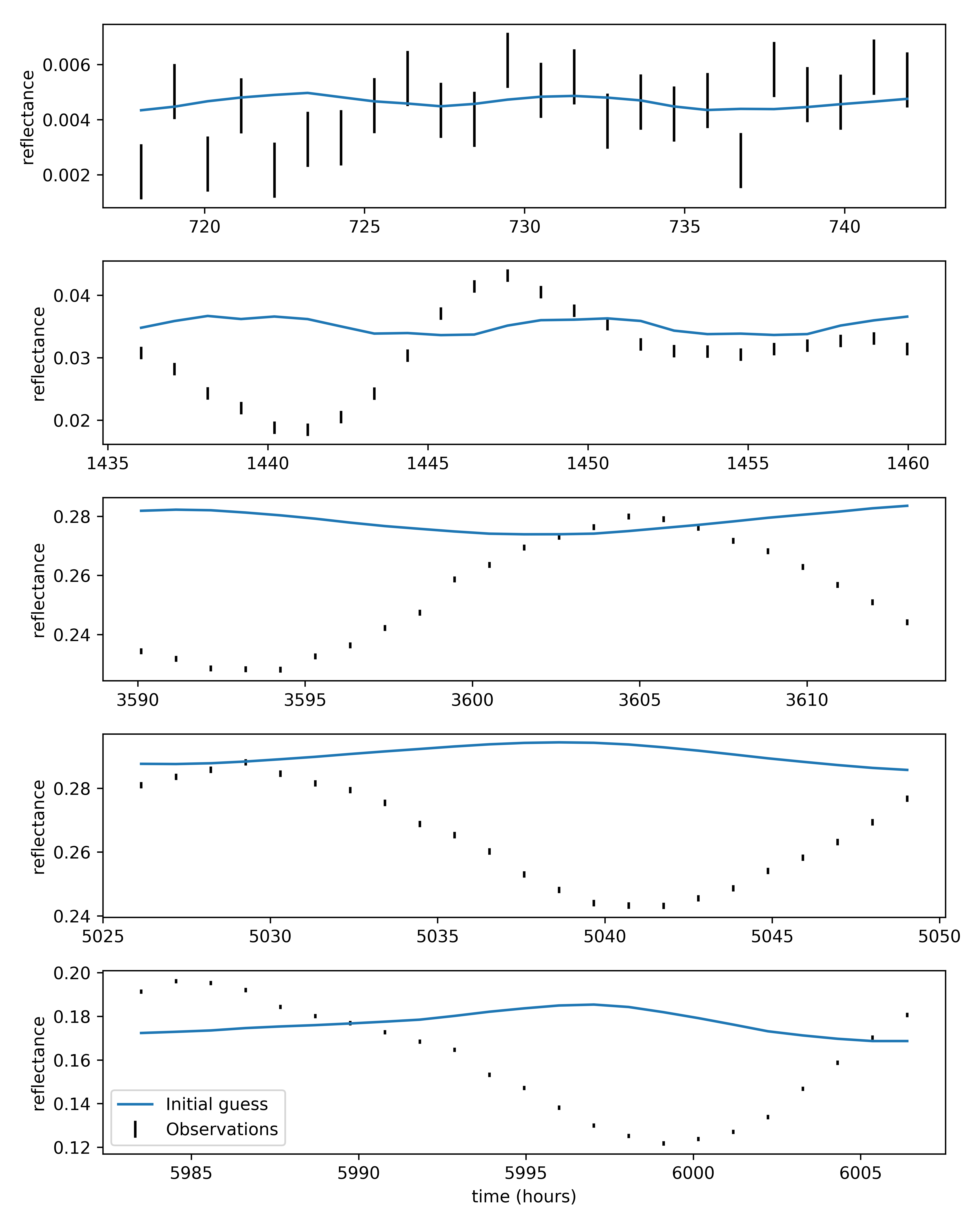
We’re not being careful with drawing initial parameters here, so make sure the log(posterior) is finite before attempting to fit the data.

Let’s see where we’re starting from:

fig, axs = plt.subplots(len(epoch_starts), 1,
                        figsize=(8, 2*len(epoch_starts)))

for ax, epoch_start in zip(axs, epoch_starts):
    sel = (logpost.times >= epoch_start) & \
            (logpost.times - epoch_start < epoch_duration)
    ax.errorbar(times[sel], logpost.reflectance[sel],
                logpost.sigma_reflectance[sel],
                capthick=0, fmt='o', markersize=0, color='k',
                label='Observations')
    ax.plot(logpost.times[sel], logpost.lightcurve(p0)[sel],
            label='Initial guess')

    ax.set_ylabel('reflectance')
axs[-1].set_xlabel('time (hours)')
axs[-1].legend(loc='lower left')

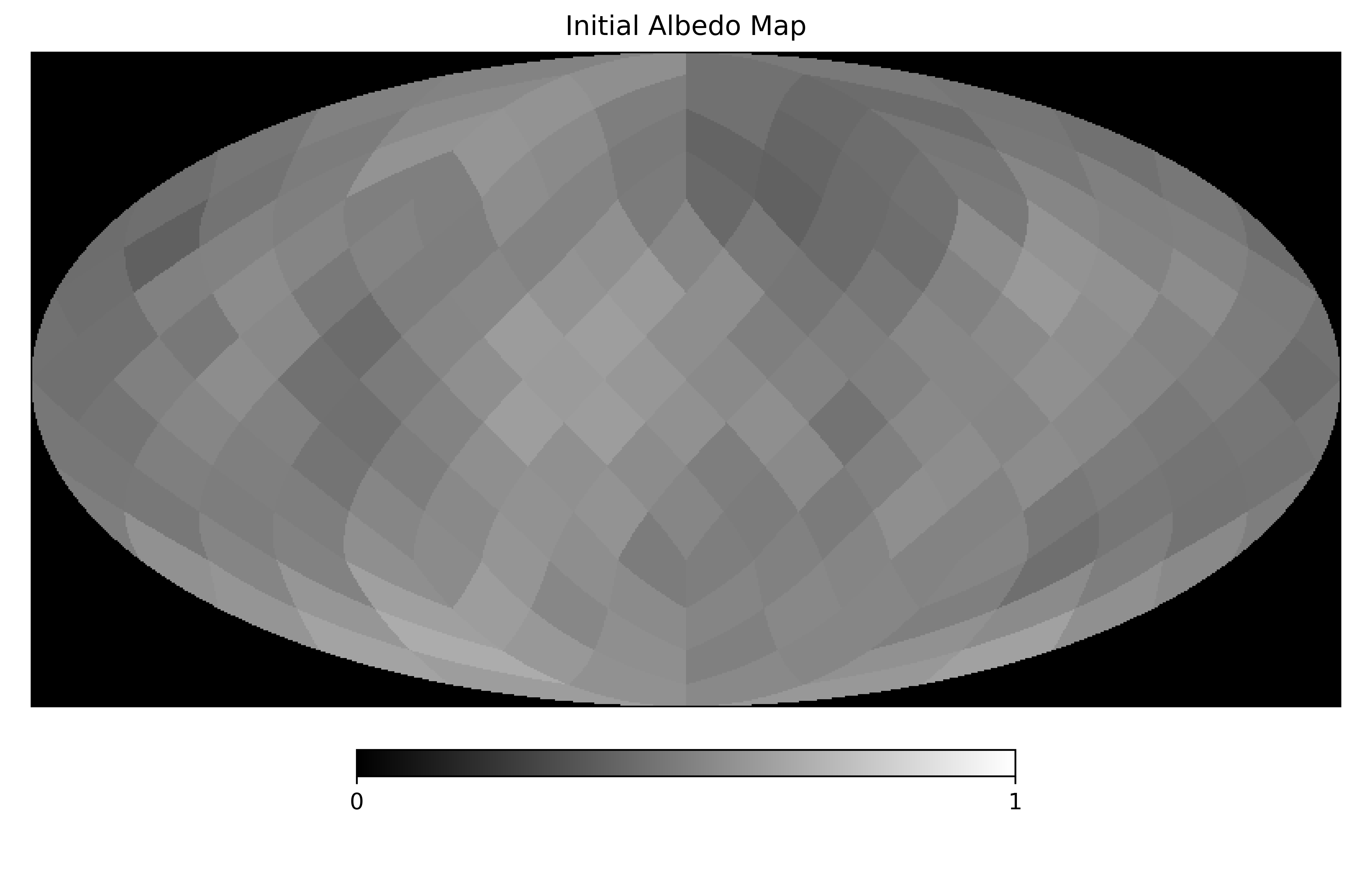
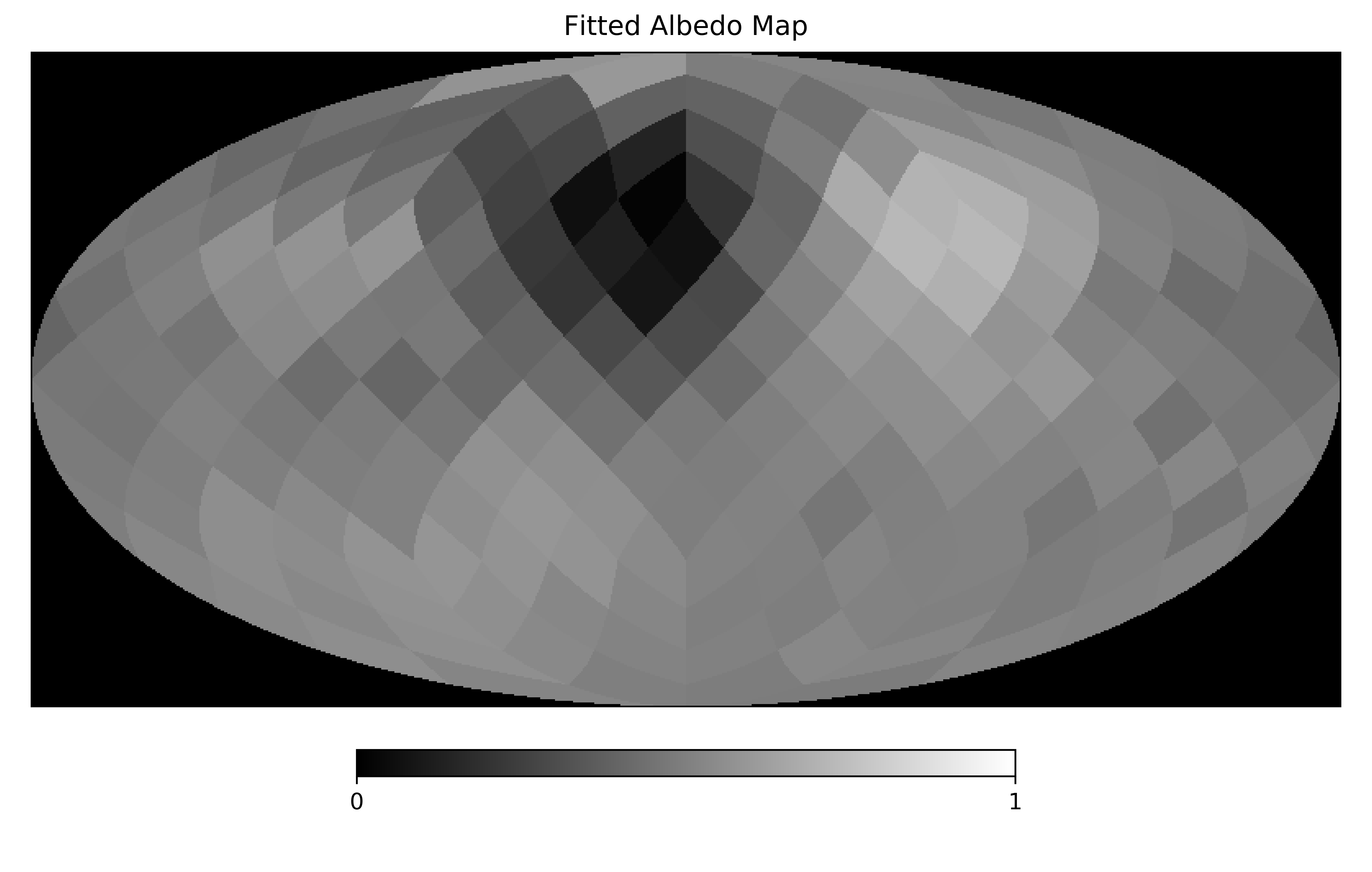
hp.mollview(logpost.hpmap(p0), min=0, max=1,
            title='Initial Albedo Map', cmap='gist_gray')

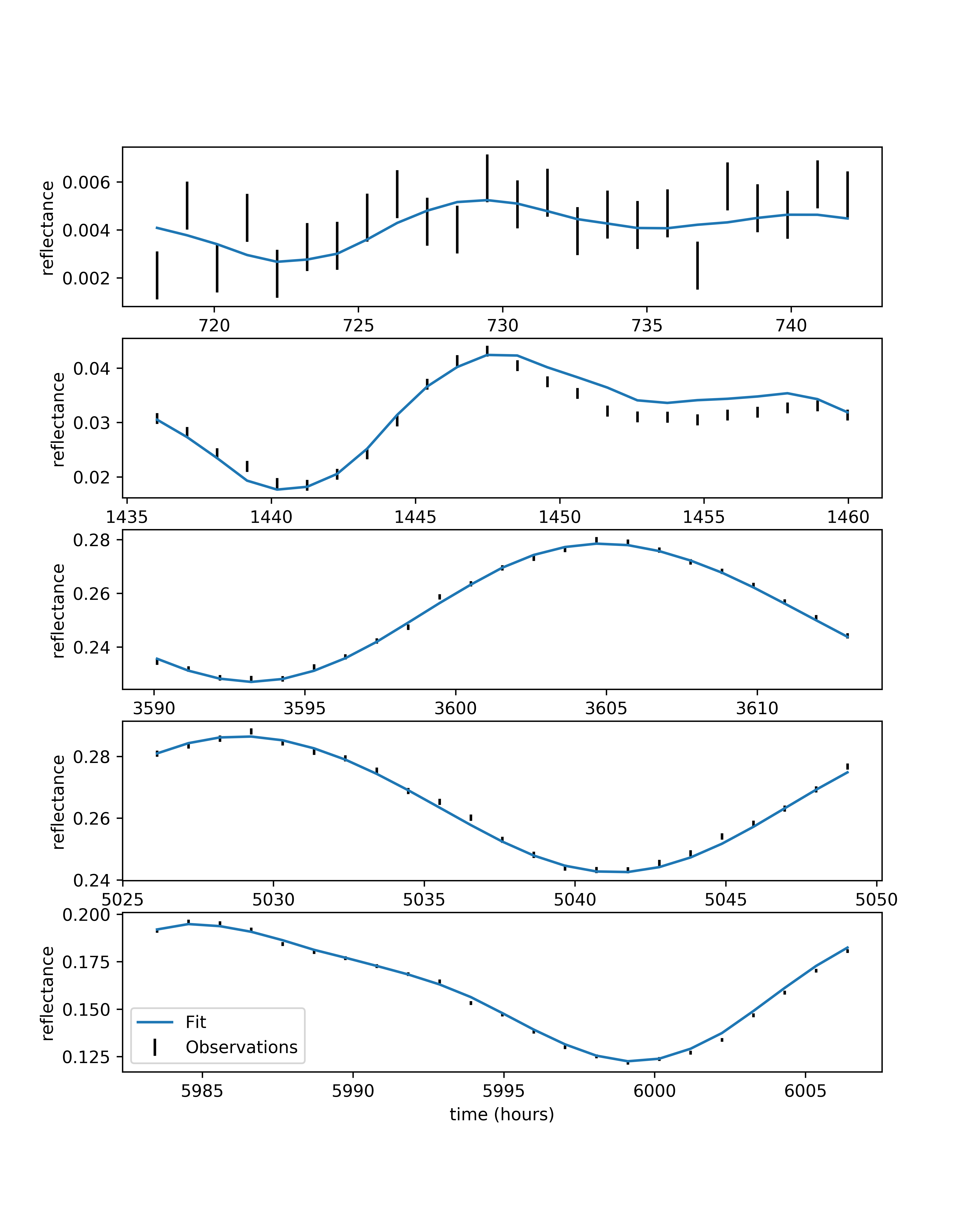
We’re finally ready to fit. For this we’ll use scipy.optimize.minimize. The posterior is high-dimensional and unlikely to be smooth. We’ve found using the BFGS and Powell methods sequentially to be reasonably efficient:

p_fit = minimize(lambda x: -logpost(x), p0, method='BFGS').x
p_fit = minimize(lambda x: -logpost(x), p_fit, method='powell',
                 options={'ftol':0.01}).x

Giving us:

There is a convenience function for doing that uses a callback function to show how the fit progresses. It can be used in a Jupyter notebook in the following way:

import exocartographer.visualize as ev
ev.inline_ipynb()

p_fit = ev.maximize(logpost, p0,
                    epoch_starts=epoch_starts,
                    epoch_duration=epoch_duration)

Due to the complexity of the problem this is almost certainly not the global maximum, and for that reason we have avoided calling this a “best” fit. This is merely meant to serve as an illustrative example for building and evaluating a posterior function, to help you work toward more robust optimization, or better yet uncertainty quantification!