Geodetic coordinates

				UTM coordinates

					srModel.u sec/km Isotropic slowness srModel.ghead srModel.ghead(1) km X-offset of u(1,1,:) wrt origin cartesian system See Coordinate System srModel.ghead(2) km Y-offset of u(1,1,:) wrt origin of cartesian system See Coordinate System srModel.ghead(3) integer Number of nodes in the x-direction also srModel.nx srModel.ghead(4) integer Number of nodes in the y-direction also srModel.ny srModel.ghead(5) integer Number of nodes in the z-direction also srModel.nz srModel.ghead(6) km Spacing of nodes in the x-direction also srModel.gx srModel.ghead(7) km Spacing of nodes in the y-direction also srModel.gy srModel.ghead(8) km Spacing of nodes in the z-direction also srModel.gz

				There are number of derived fields for the srModel structure.  The ones defined in the generic set are present for all models, whether or not water-path corrections are applied or other optional fields are used.  Some of these may take up memory, so carrying them around to all functions might not be advised.  Fields can be removed using the rmfield command.

					srModel.nx srModel.ny srModel.nz integer srModel.ghead(3:5) srModel.gx srModel.gy srModel.gz km srModel.ghead(6:8) srModel.nodes integer Total number of nodes (nx*ny*nz) srModel.xg srModel.yg srModel.zg km Vectors storing x y and z values of nodes. Elevation is not included in these values; z value is model z-value as described in coordinate system. srModel.zg is relative to top surface of velocity model; z is positive upward. Matlab command: srModel.xg=linspace(srModel.ghead(1), srModel.ghead(1)+ (srModel.nx(1)*srModel.gx,srModel.nx)’; srModel.XG srModel.YG km Matrix of x and y graph locations.  See meshgrid in matlab. srModel.LON srModel.LAT decimal degrees Matrix of longitude and latitude positions that define the location of vertical columns of srModel.u srModel.elevation kilometers Elevation to top layer of nodes that define the slowness model. Can be plotted: cartesian coordinates:      pcolor(srModel.xg, srModel.yg, srModel.elevation) geographic coordinates:  pcolor(srModel.LON,srModel.LAT,srModel.elevation) minx, maxx miny, maxy minz, maxz km xyz limits of slowness graph in cartesian coordinate system

					When waterpath corrections are required for airgun data (see the srControl structure), the function load_srModel derives a “seafloor” interface field and includes it in srModel.  This is a derived sub-structure of srModel, i.e., let the code fill it in.  The seafloor interface is derived from srElevation. srModel.interface.id integer Unique interface id srModel.interface.name character (cell array) {‘seafloor’ } (NOTE: must be cell array) srModel.interface.X km Array of x-locations of grid points defining interface.  Size of X and Y must be identical. srModel.interface.Y km Array of y-locations of grid points defining interface. Size of X and Y must be identical. srModel.interface.elevation km Elevation of seafloor at XY array locations

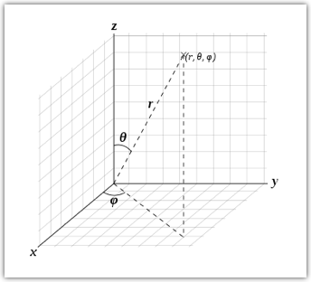
					Anisotropy at a node is defined in spherical coordinates (r, θ, φ) where r is the percentage of anisotropy, θ is the zenith angle from the positive z-axis to the point, and φ is the azimuth angle from the positive x-axis to the orthogonal projection of the point in the x-y plane; see figure below. If your model is isotropic (and srControl.tf_anisotropy=0), there is no need to define these fields. srModel.anis_fraction unitless Fraction of anisotropy (e.g., 0.06 is 6%) srModel.anis_theta radians θ is the zenith angle from the +z axis to the point; see figure. srModel.anis_phi radians φ is the azimuth angle from the positive x-axis to the orthogonal projection of the point in the x-y plane. Positive φ is in the +x, +y direction. srModel.anis_A unitless Scale term for azimuthal anisotropy.  See Eqn. A1 of Dunn et al., 2005 srModel.anis_B unitless Scale term for azimuthal anisotropy.  See Eqn. A1 of Dunn et al., 2005

					Interfaces can be included in the velocity model allowing analysis of secondary arrivals  (e.g., PmP).  An interface is an optional field, meaning that it must be defined by the user.  Note that the seafloor interface used for waterpath corrections is a derived field, not an optional field.  The seafloor interace is discussed above (Derived Fields:  Waterpath corrections). srModel.interface.id integer Unique interface id. srModel.interface.name character (cell array) Name of the interface causing either reflection or conversion.  NOTE:  Must be cell array, e.g. {‘Moho’}. srModel.interface.X km 2D matrix specifying x points at which the Z data is given.  Size of X, Y, Z must be identical. Defined in local cartesian coordinates. srModel.interface.Y km 2D matrix specifying y points at which the Z data is given. Size of X, Y, Z must be identical. Defined in local cartesian coordinates. srModel.interface.Z km The model z-value of the interface at the points in matrices X and Y. Defined in local cartesian coordinates. srModel.interface.elevation km Elevation of the interface at the points in matrices X and Y. srModel.interface(1)              id: 1            name: {‘moho’}               X: [551x141 double]               Y: [551x141 double]               Z: [551x141 double]       elevation: [551x141 double]     indiceAbove: [77691x1 double]     indiceBelow: [77691x1 double]         Normalx: [551x141 double]         Normaly: [551x141 double]         Normalz: [551x141 double]srModel.interface(1) =

				Several derived fields are useful for calculating partial derivatives srModel.interface.indiceAbove integer Nodal indice above the interface at (i,j) location srModel.interface.indiceBelow integer Nodal indice below the interface at (i,j) location srModel.interface.Normalx unitless Component of unit vector normal to the interface at (i,j) location srModel.interface.Normaly unitless Component of unit vector normal to the interface at (i,j) location srModel.interface.Normalz unitless Component of unit vector normal to the interface at (i,j) location

				The definition of anisotropy in Stingray differs from hpt (theta and phi are switched in hpt and not consistent with conventional notation).

				oldmodel