|
|
|
|
 | MAGNETICS
This appendix contains the following sections:
|
|
|
|
 |
|
|
3. | Processing Methodology
|
|
|
|
|
|
 | Filtering and quality control
|
|
|
|
|
|
| Background magnetic field removal
|
|
|
|
|
|
| Ship magnetic field removal
|
|
|
|
|
|
| The magnetic field was recorded using a GeoMetrics 882 magnetometer towed nominally 60 meters astern of the vessel on starboard side. Data was logged to the LDEO data logging system. The system performed well during the survey. Approximately 1,380,000 points of data were collected.
Instrument: GeoMetrics 882 Cesium Marine Magnetometer System Specifications
Operating Principle: Self-oscillating split-beam Cesium Vapor (non-radioactive)
Operating Range: 20,000 to 100,000 nT
Operating Zones: The earth’s field vector should be at an angle greater than 6° from the sensor’s equator and greater than 6° away from the sensor’s long axis. Automatic hemisphere switching is standard.
CM-221 Counter Sensitivity: <0.004 (nT/πHz) rms. Up to 10 samples per second
Heading Error: ±1 nT (over entire 360° equatorial and polar spin)
Absolute Accuracy: <3 nT throughout range
Output: RS-232 at 1,200 to 19,200 Baud
Mechanical: Sensor Fish: Body 2.75 in. (7 cm) dia., 4.5 ft (1.37 m) long with fin assembly (11 in. cross width), 40 lbs. (18 kg) Includes Sensor and Electronics and 1 main weight. Additional collar weights are 14lbs (6.4kg) each, total of 5 capable
Tow Cable: Kevlar Reinforced multiconductor tow cable. Breaking strength 3,600 lbs, 0.48 in OD, 200 ft maximum. Weighs 17 lbs (7.7 kg) with terminations.
Operating Temperature: -30°F to +122°F (-35°C to +50°C)
Storage Temperature: -48°F to +158°F (-45°C to +70°C)
Water Tight: O-Ring sealed for up to 9000 ft (2750 m) depth operation
Instrument Location: The towfish was an approximate 60 m behind the NRP (navigation reference point where the vessel position is resolved) as detailed in the Offsets Configuration file (Attachment 4).
|
|
|
|
 |
|
|
| 3. Processing Methodology:
Data processing was completed using a series of Matlab functions and script files (see schematic, fig. 1). All processing was completed through the header function UpdateAll (Attachment 1). Each step of processing is outlined below.
|
|
|
|
 |
|
|
| 
Figure 1. Schematic of Matlab files used during magnetic data processing steps.
|
|
|
|
|
|
| Collection: Raw magnetic (date, time, field strength) and CNav navigation (date, time, latitude, longitude, heading) data was collected from each separate day of the cruise (Attachments 2, 3, 4). Afterwards, data from the separate days were formatted and combined to a single magnetic and navigation table (Attachments 5, 6, 7 8). Main formatting at this stage involved converting the date and time format of the raw data (Year, Yearday, Hour, Minute, Second) to a serial date format.
|
|
|
|
|
|
| Merging: Raw magnetic data was merged with the CNav navigation data using the serial date data field (Attachment 9). Since the magnetic and navigation data were collected at separate frequencies (0.1 and 1 Hz, respectively), data was matched to the closest second.
|
|
|
|
|
|
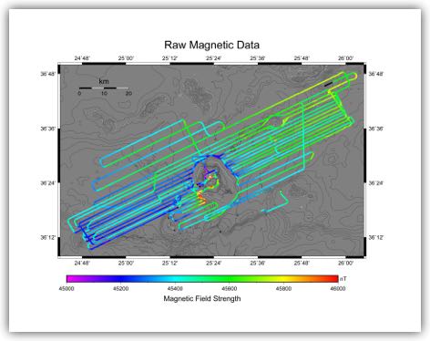
| Filtering and Quality Control: Data was automatically checked for missing or erroneous values which fell outside 0.4 standard deviation away from the mean (Attachment 10). Afterwards, high-frequency features were filtered out of the data using a 10m moving- window average (Attachment 11).
|
|
|
|
|
|
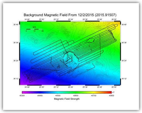
| Background Magnetic Field Removal: We estimated the background magnetic field during the cruise using the International Geomagnetic Reference Field 2012 (IGRF 2012) model and a predictive model of the secular variation for adjusted dates between 2015 and 2020. We created a 10m grid of background magnetic variation using the midway cruise date (12/2/15, 2015.91507) and subtracted it from the raw data (Attachment 12). Values in the grid ranged [45310, 45734] nT (fig. 2). Across the cruise dates (11/22/15 – 12/15/15), the magnetic field at the grid boundaries (latitude: [24.7353, 26. 0488], longitude: [24.7353, 26.7353]) varied <3 nT.
|
|
|
|
|
|
| Ship Magnetic Field Removal: Using the method of Buchanan et al. (1996), we further corrected the data by removing the ship’s magnetic field (Attachment 13). The magnetic field of the ship (f_s) at a given heading (in azimuth) is given by the equation:
f_s=a_1+ a_2 cos〖(h+θ)〗+ a_3 cos〖(2 (h+ θ))〗 (1)
Where h is the ship heading, θ is the angle of the magnetometer relative to the ship, and a_1, a_2, and a_3 are constant coefficients. From the raw magnetic field with the background signal removed, we collected the mean and standard deviation of field values over 2 degrees of heading from measurements located away from the Santorini caldera to remove bias from extreme maxima and minima (fig. 3, black dots). Using the mean and standard deviation values (fig. 3, white diamonds, purple lines, respectively), we used a least squares approach to calculate the coefficients a_1, a_2, and a_3. Afterwards, we fit different values of θ to the equation to find the value that best shifted the curve to match the data. The least squares method found coefficient values of -55.9669, -116.7476, and 42.7715, respectively, after three iterations with a relative residual of 6.3 x10⁻¹⁵. Furthermore, we found a θ value of -8° best matches the observed data (fig. 3, green line). Thus, our corrections for ship magnetic field are defined by the equation:
f_s=-55.9669- 116.7476 cos(h-8)+ 42.7715 cos〖(2 (h- 8))〗 (2)
For each data measurement, the ship’s magnetic field was calculated from the measurements heading and was subsequently removed.
|
|
|
|
|
|
|
| 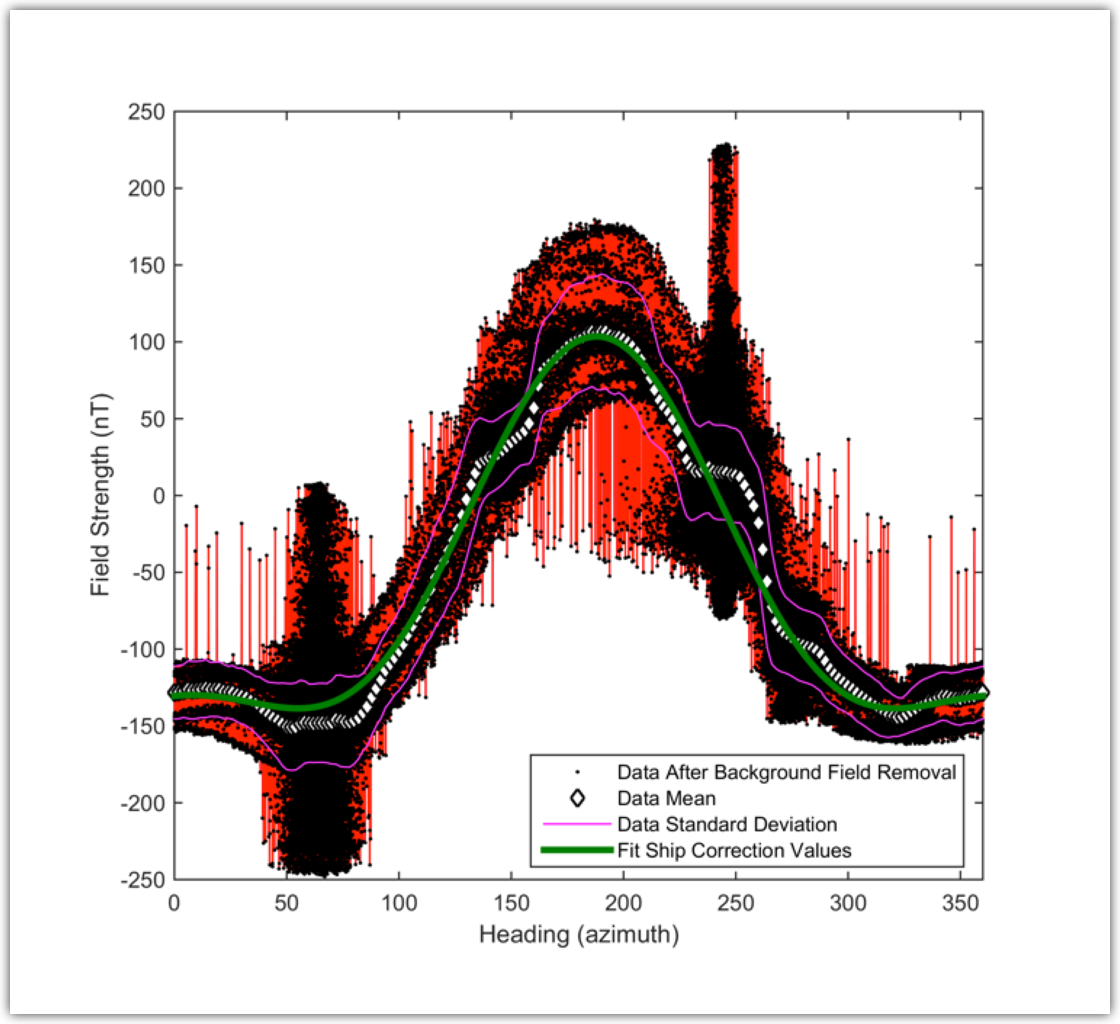
Figure 2. Ship magnetic field correction. Black dots with red lines are raw data with background field removed. White diamonds are mean field strength taken at 2° intervals with standard deviation above and below the mean given by purple lines. Green line is the fit to the data using equation (2).
|
|
|
|
|
|
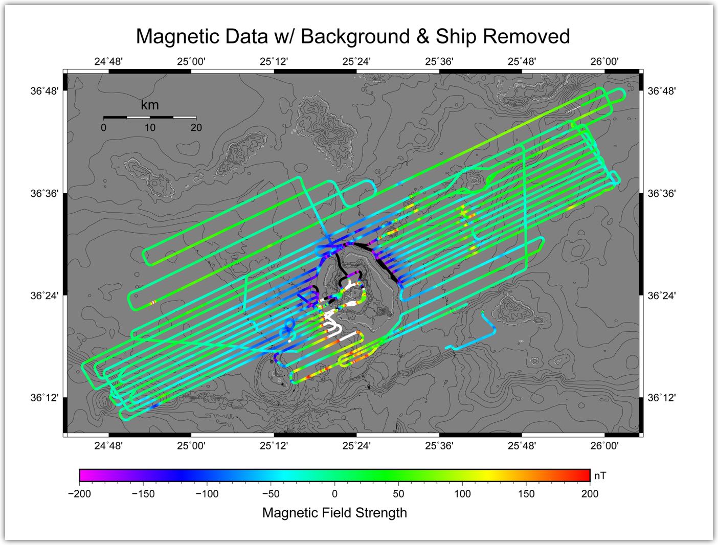
| Final data and output: The final data contains the navigation position and the corrected total field readings after background and ship magnetic field correction in one second intervals matched to the navigation GPS timestamp at the nearest second. The latitude, longitude, and total field strength is then output to data files to use in map generation (Attachement 14).
|
|
|
|
|