3D field line/stream plots in Mathematica

This is the HTML version of a Mathematica 8 notebook. You can copy and paste the following into a notebook as literal plain text. For the motivation and further discussion of this notebook, see the discussion on StackExchange. If you want to plot 3D fields using vectors instead of field lines, look at the Mathematica graphics main page instead.

gradientFieldPlot

The main function on this page is fieldLinePlot, but I have split it into two functions to be more modular. Also, the problem of where to start drawing the field lines is treated separately because it depends a lot on the particular application.

• fieldSolve[f,x,x0,Subscript[t, max]] symbolically takes a vector field f with respect to the vector variable x, and then finds a vector curve r[t] starting at the point x0 satisfying the equation dr/dt=α f[r[t]] for t=0...tmax. Here α=1/|f[r[t]]| for normalization. To get verbose output add debug=True to the parameter list.

• fieldLinePlot[field,varlist,seedList] plots 3D field lines of a vector field (first argument) that depends on the symbolic variables in varlist. The starting points for these variables are provided in seedList.

Each element of seedList={{p1, T1},{p2, T2}...} is a tuple where pi is the starting point of the i-th field line and Ti is the length of that field line in both directions from p_i.

fieldSolve::usage = 
  "fieldSolve[f,x,x0,\!\(\*SubscriptBox[\(t\), \(max\)]\)] \
symbolically takes a vector field f with respect to the vector \
variable x, and then finds a vector curve r[t] starting at the point \
x0 satisfying the equation dr/dt=\[Alpha] f[r[t]] for \
t=0...\!\(\*SubscriptBox[\(t\), \(max\)]\). Here \[Alpha]=1/|f[r[t]]| \
for normalization. To get verbose output add debug=True to the \
parameter list.";

fieldSolve[field_, varlist_, xi0_, tmax_, debug_: False] := Module[
  {xiVec, equationSet, t},
  If[Length[varlist] != Length[xi0], 
   Print["Number of variables must equal number of initial conditions\
\nUSAGE:\n" <> fieldSolve::usage]; Abort[]];
  xiVec = Through[varlist[t]];
  (*// Below, Simplify[equationSet] would cost extra time and doesn't help with the numerical solution, so don't try to simplify. *)
  
  equationSet = Join[
    Thread[
     Map[D[#, t] &, xiVec] == 
      Normalize[field /. Thread[varlist -> xiVec]]
     ],
    Thread[
     (xiVec /. t -> 0) == xi0
     ]
    ];
  If[debug, 
   Print[Row[{"Numerically solving the system of equations\n\n", 
      TraditionalForm[(Simplify[equationSet] /. t -> "t") // 
        TableForm]}]]];
  (*// This is where the differential equation is solved. *)
  (*// The Quiet[] command suppresses warning messages because numerical precision isn't crucial for our plotting purposes: *)
  
  Map[Head, First[xiVec /.
     Quiet[NDSolve[
       equationSet,
       xiVec,
       {t, 0, tmax}
       ]]], 2]
  ]

fieldLinePlot::usage = "fieldLinePlot[field,varlist,seedList] plots \
3D field lines of a vector field (first argument) that depends on the \
symbolic variables in varlist. The starting points for these \
variables are provided in seedList. Each element of \
seedList={{\!\(\*SubscriptBox[\(p\), \(1\)]\), \!\(\*SubscriptBox[\(T\
\), \(1\)]\)},{\!\(\*SubscriptBox[\(p\), \(2\)]\), \
\!\(\*SubscriptBox[\(T\), \(2\)]\)}...} is a tuple where \
\!\(\*SubscriptBox[\(p\), \(i\)]\) is the starting point of the i-th \
field line and \!\(\*SubscriptBox[\(T\), \(i\)]\) is the length of \
that field line starting from \!\(\*SubscriptBox[\(p\), \(i\
\)]\).";

fieldLinePlot[field_, varList_, seedList_, opts : OptionsPattern[]] :=
  Module[{sols, localVars, var, localField},
  If[Length[seedList[[1, 1]]] != Length[varList], 
   Print["Number of variables must equal number of initial conditions\
\nUSAGE:\n" <> fieldLinePlot::usage]; Abort[]];
  localVars = Array[var, Length[varList]];
  localField = 
   ReleaseHold[
    Hold[field] /. 
     Thread[Map[HoldPattern, Unevaluated[varList]] -> localVars]];
  (* // Assume that each element of seedList specifies a point AND the length of the field line: *)
  Show[ParallelTable[
    (
      ParametricPlot3D[
        Evaluate[Through[#[t]]], {t, #[[1, 1, 1, 1]], #[[1, 1, 1, 2]]},
        Evaluate@
         Apply[Sequence, 
          FilterRules[{opts}, Options[ParametricPlot3D]]]] &
      )@
     fieldSolve[localField, localVars, seedList[[i, 1]], 
      seedList[[i, 2]]]
    , {i, Length[seedList]}]]
  ];
Options[fieldLinePlot] = Options[ParametricPlot3D];
SyntaxInformation[
   fieldLinePlot] = {"LocalVariables" -> {"Solve", {2, 2}}, 
   "ArgumentsPattern" -> {_, _, _, OptionsPattern[]}};
SetAttributes[fieldSolve, HoldAll];
    

Example 1

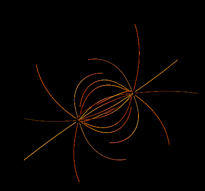
Coulomb field of two equal charges at r = 0 and r = {1, 1, 1}:

seedList = 
  With[{vertices = .1 N[PolyhedronData["Icosahedron"][[1, 1]]]}, 
   Join[Map[{#, 2} &, vertices], 
    Map[{# + {1, 1, 1}, -2} &, vertices]]];

Show[fieldLinePlot[{x, y, z}/
    Norm[{x, y, z}]^3 - ({x, y, z} - {1, 1, 1})/
    Norm[{x, y, z} - {1, 1, 1}]^3, {x, y, z}, seedList, 
  PlotStyle -> {Orange, Specularity[White, 16], Tube[.01]}, 
  PlotRange -> All, Boxed -> False, Axes -> None], 
 Background -> Black]
  

Example 2

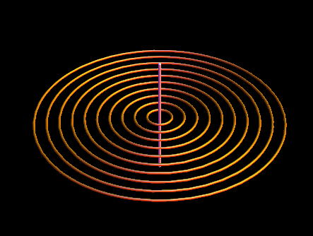
Magnetic field of an infinite straight wire:

With[{seedList = Table[{{x, 0, 0}, 6.5}, {x, .1, 1, .1}]
  },
 Show[fieldLinePlot[{-y, x, 0}/(x^2 + y^2), {x, y, z}, 
   seedList, PlotStyle -> {Orange, Specularity[White, 16], Tube[.01]},
    PlotRange -> All, Boxed -> False, Axes -> None], 
  Graphics3D@Tube[{{0, 0, -.5}, {0, 0, .5}}], Background -> Black]]