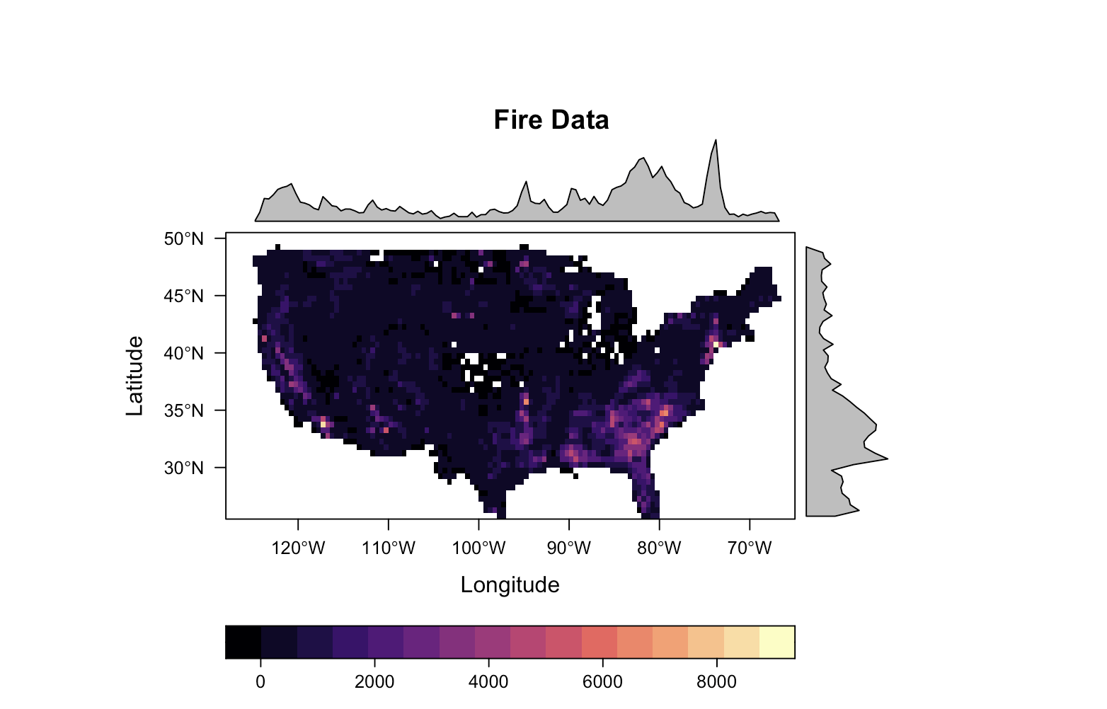
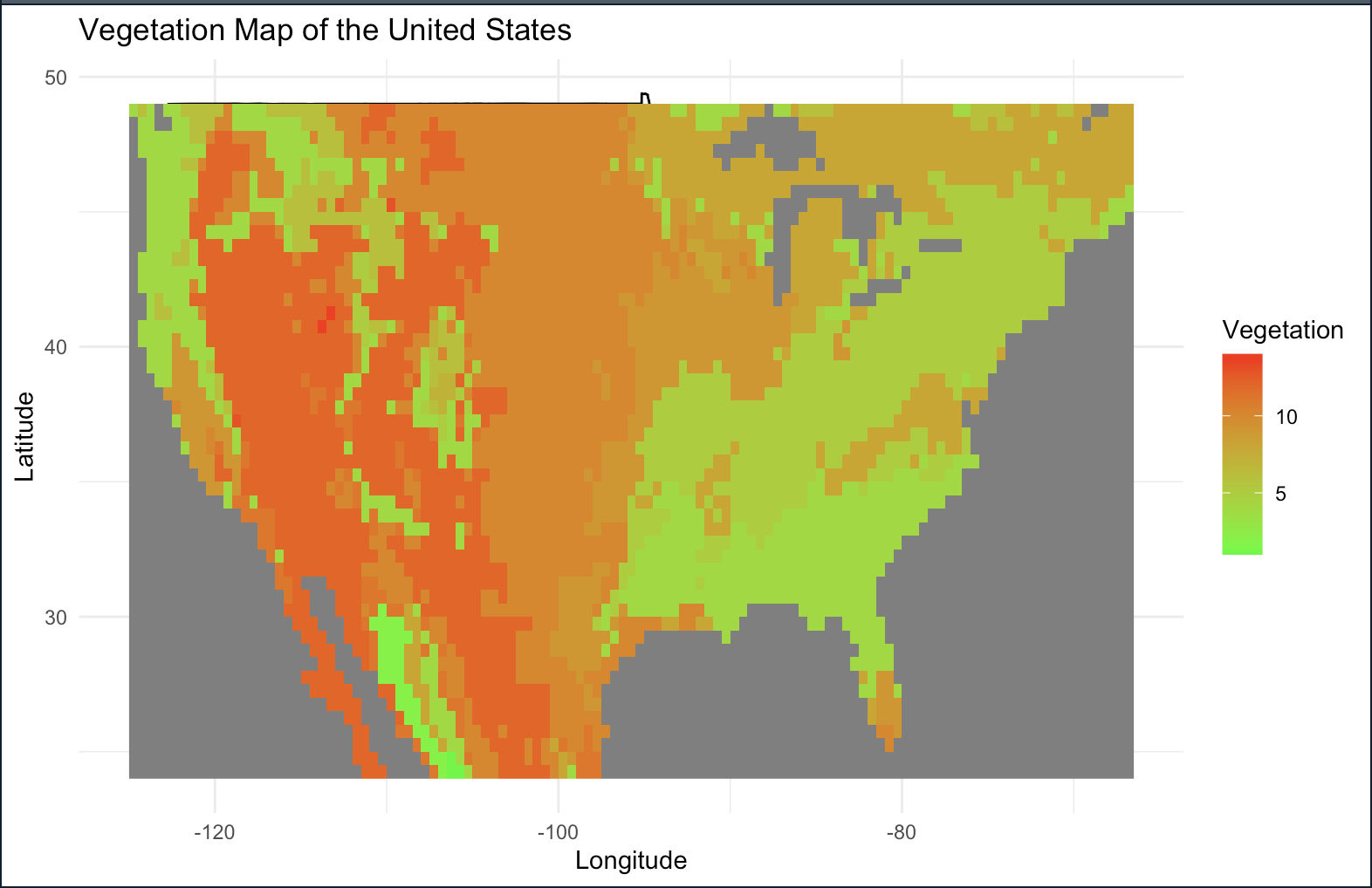
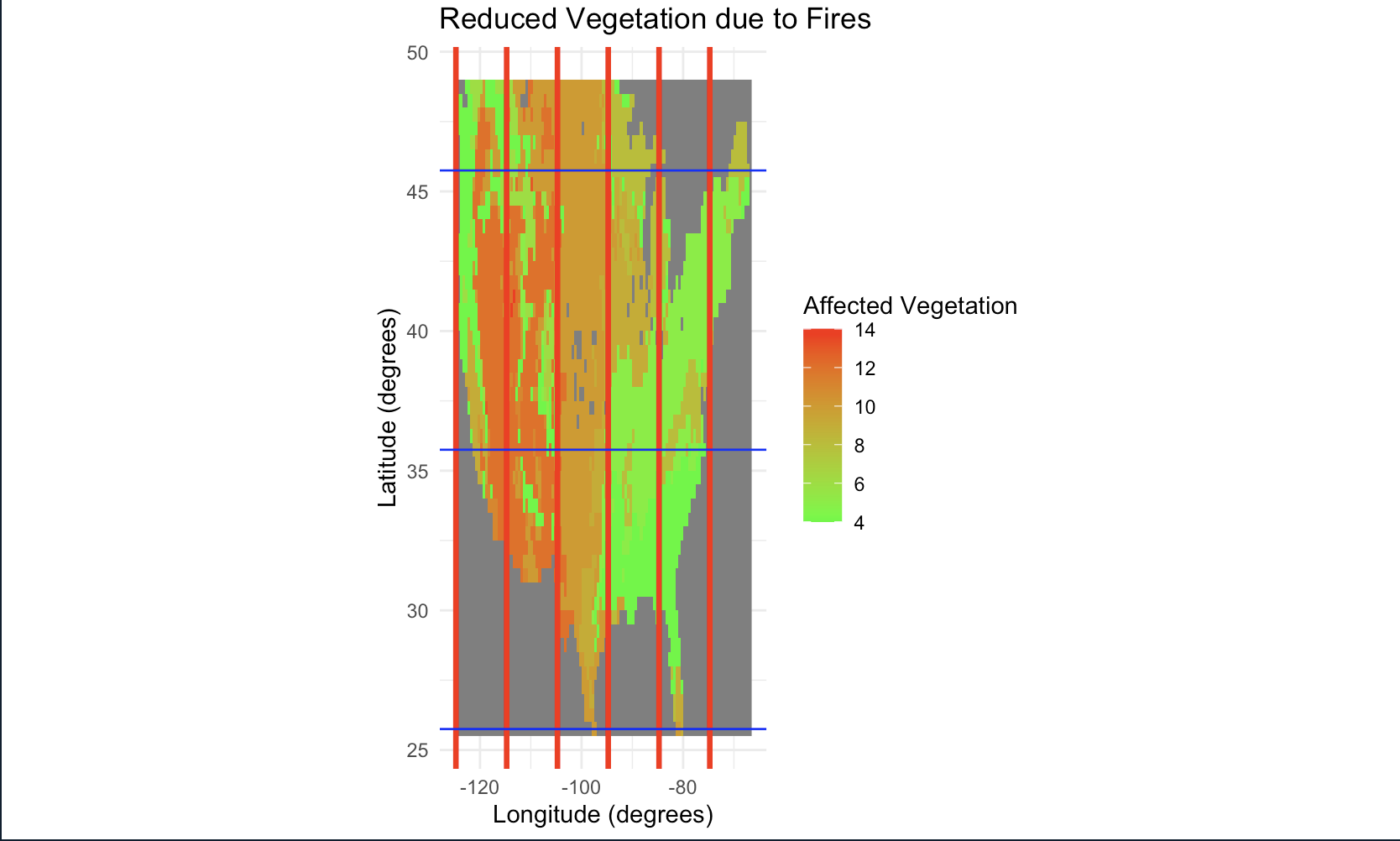
Fire devastates vegetation by consuming vast amounts of plant matter, leaving behind barren landscapes devoid of life. It ravages ecosystems, destroying habitats and disrupting the delicate balance of nature. The reduction in vegetation leads to soil erosion, loss of biodiversity, and increased vulnerability to erosion and other environmental threats. This can be seen in the maps above.
    install.packages("raster")
    install.packages("ncdf4")
    install.packages("rasterVis")
    install.packages("ggplot2")

    library(rasterVis)
    library(raster)
    library(ncdf4)
    library(ggplot2)
    library(maps)

    setwd("/Users/tessawright/Documents/geog490/data/")

    veg_data <- nc_open("sage_veg30.nc")
    fire_data <- nc_open("us_fires.nc")

    print(veg_data)
    print(fire_data)

    veg_data <- raster("sage_veg30.nc")
    fire_data <- raster("us_fires.nc")

    levelplot(veg_data, main = "Vegetation Data")
    levelplot(fire_data, main = "Fire Data")

    us_extent <- extent(-125, -66.5, 24, 49)
    veg_data_us <- crop(veg_data, us_extent)
    fire_data_us <- crop(fire_data, us_extent)

    fire_data_binary <- as.integer(fire_data_us > 0)

    affected_veg <- veg_data_us * fire_data_binary

    affected_veg_df <- as.data.frame(affected_veg, xy = TRUE)
    names(affected_veg_df) <- c("x", "y", "affected_veg")

    longitude_lines <- data.frame(x = seq(-180, 180, by = 10), y = 0)
    latitude_lines <- data.frame(x = 0, y = seq(-90, 90, by = 10))

    veg_data_df <- as.data.frame(veg_data_us, xy = TRUE)
    names(veg_data_df) <- c("lon", "lat", "vegetation_value")
    us_map <- map_data("state")
    us_veg_map <- ggplot() +
      geom_map(data = us_map, map = us_map,
               aes(x = long, y = lat, map_id = region),
               fill = "white", color = "black") +
      geom_raster(data = veg_data_df, aes(x = lon, y = lat, fill = vegetation_value)) +
      scale_fill_gradient(name = "Vegetation", low = "green", high = "red") +
      labs(title = "Vegetation Map of the United States",
           x = "Longitude", y = "Latitude") +
      theme_minimal()
    print(us_veg_map)


    affected_veg_plot <- ggplot(affected_veg_df, aes(x = x, y = y, fill = affected_veg)) +
      geom_raster() +
      scale_fill_gradient(name = "Affected Vegetation", low = "green", high = "red") +
      labs(title = "Reduced Vegetation due to Fires",
           x = "Longitude (degrees)",
           y = "Latitude (degrees)") +
      theme_minimal() +
      coord_fixed(ratio = 5.5)
    lon_range <- range(affected_veg_df$x)
    lat_range <- range(affected_veg_df$y)

    lon_line_size <- diff(lon_range) / 50 # Adjust 50 as needed for line density
    lat_line_size <- diff(lat_range) / 50
    affected_veg_plot <- affected_veg_plot +
      geom_vline(xintercept = seq(lon_range[1], lon_range[2], by = 10), color = "red", size = lon_line_size) +
      geom_hline(yintercept = seq(lat_range[1], lat_range[2], by = 10), color = "blue", size = lat_line_size)
    print(affected_veg_plot)

    ggsave("combined_plot.png", plot = affected_veg_plot, width = 10, height = 6, units = "in", dpi = 300)
    ggsave("us_vegetation_map.png", plot = us_veg_map, width = 10, height = 6, units = "in", dpi = 300)