Future Climate Analogue Mapping -- Directions
Two Steps: 1) Select specific analogue
parameters; 2) Click on a location
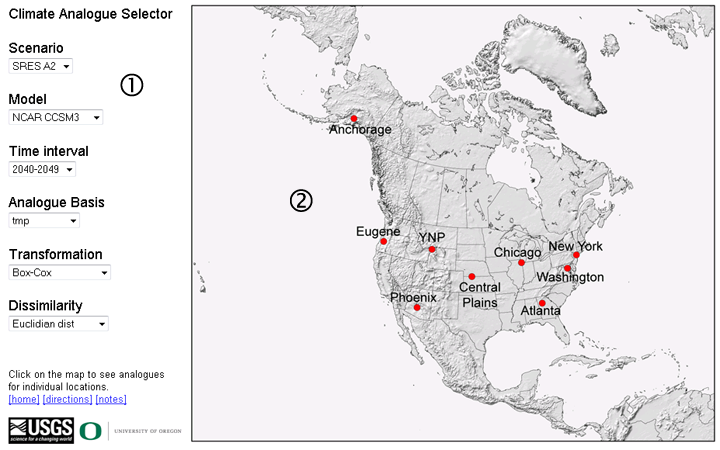
On the Analogue Selector page, first select the specific analogue
parameters such as the model, analogue basis (which climate variables
are used), and so on using the drop-down boxes on the left (1), and
then click on a location hot spot on the map on the right (2).
Analogue maps
The first map that will appear shows on the left the future locations of the present climate at the point (where the present climate is going), while the map on the right shows the present locations of the future climate of at the point (where the future climate is coming from). See the notes for a discussion of the color scheme used to indicate the "strength" of the analogue: smaller dissimilarities (i.e. similar climate) are plotted in dark red, while larger dissimilarities are plotted in light red.
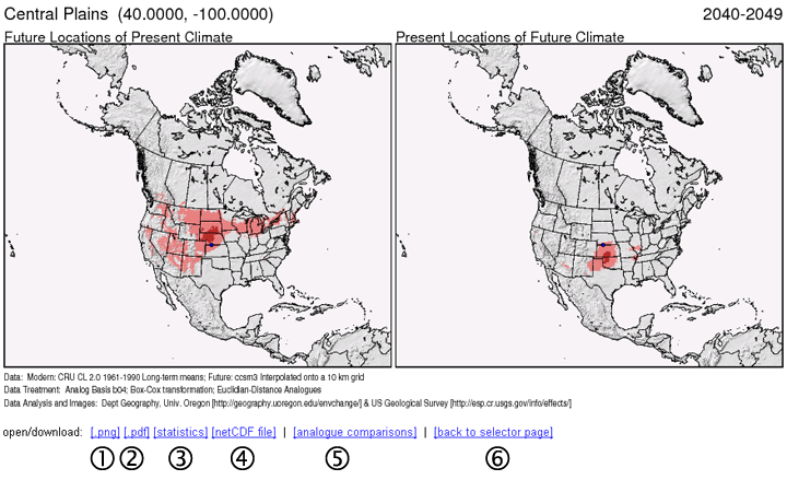
The links at the bottom of the above set of maps open other images, a table of information about the climate of the analogue points, the dissimilarity values, and can also be used to navigate back to the selector page, as follows:
(1) opens a higher resolution .png image in the brower that can be panned and scrolled;
(2) opens a .pdf of the image;
(3) opens a table of information about the climate of the analogue points (see below);
(4) opens or downloads the netCDF file of analogues. This file can be opend and viewed in Panoply (see below);
(5) links to a second set of maps that show points with similar climates to the target point;
(6) navigates back to the selector page with the default settings. To get back to the selector page with the current settings preserved, use the browser back arrow.
The second set of analogue maps shows the similarity between the present climate at the target point and present climate elsewhere (left), and between the future climate at the target point and future climate elsewhere (right). These maps can be used to infer the representativeness of the present and future climates at the target point.
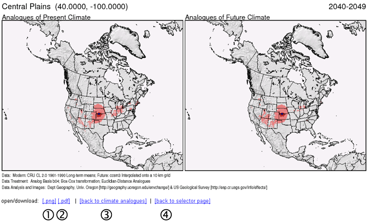
The links at the bottom of this second set of maps do the following:
(1) opens a higher resolution .png image in the browser which can be panned and scrolled
(2) opens a .pdf of the image
(3) navigates back the first set of maps
(4) navigates back to the selector page with the default settings. To get back to the selector page with the current settings preserved, use the browser back arrow.
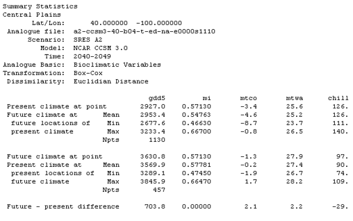
Link (3) on the first set of maps opens a table that shows the present and simulated future climate at the target point (for a particular scenario, model, time and analogue calculation method), and also shows the mean, maximum, and minimum of the climate variable values for the "strong" (1st-percentile) analogues shown in red on the maps. In some cases there may not be any strong analogues, in which case 9999s are displayed.
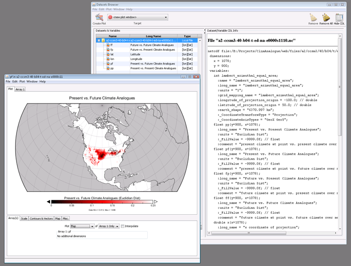
NetCDF files
The analogues are stored in netCDF files that can be downloaded and opened in (e.g.) Panoply http://www.giss.nasa.gov/tools/panoply/ The following image shows the netCDF for this example open in Panoply. To duplicate the map projection being used here, select the Azimuthal Equal-Area Projection, with the map center at -100(W) and +50(N), a radius of 42 degrees, and filled corners.