Analogue Calculations

Analogues are displayed here using statistical distance or dissimilarity measures, where low distances or dissimilarities indicate similar or analogous climates.  For each particular target point, four sets of analogues were obtained for each combination of climate scenario (and time) and choice of analogue-calculation parameters (see below):  1)  “present vs. future” analogues that show the dissimilarity between the present climate at a target point and the future climates over the “field” of grid points; these show where the present climate of the target point will occur in the future; 2) “future vs. present” analogues that show the dissimilarity between the future climate at a target point and the present climate over the field of grid points; these show where the future climate at the target point occurs at present; 3) “present vs. present” analogues that show the locations with present-day climates similar to those at the target point; and 4) “future vs. future” analogues that show the same thing under a particular future climate scenario.  These last two analogue patterns describe how unique or common the climate at a target point is at present, and how that pattern may change in the future.  Each set of four dissimilarity-value maps were also stored as netCDF files, about 31 Mbytes in size.

Analogue Bases

The calculation of dissimilarities between climates at different locations or times requires the specification of a particular set of climate variables to use.  Analogues could be expressed, for example, in terms of temperature alone, moisture alone, temperature and moisture, and so on, where the specific set of variables used is referred to here as an “analogue basis.”  Six analogue bases are used here:

Transformation of Variables

The individual climate variables have several different of kinds distributions, ranging from those that are nearly normal (e.g. temperature variables) to those that are positively skewed (long right tail, e.g. precipitation), to those with unusually shaped distributions (e.g. AE/PE, which is negatively skewed, i.e., with a long left tail).  Skewness influences the calculation of analogues by giving observations in the tails of skewed distributions disproportionally large (e.g. in the case of the upper tail of positively skewed distributions) contributions to the dissimilarity values, and those in the opposite tail disproportionally small contributions.  Individual dissimilarity values may therefore be influenced more by where an observation of a particular climate variable falls under its distribution than by practical differences in the climates of two locations. 

Consequently, the Box-Cox transformation, a variance-stabilizing power transformation, was used to transform the individual variables.  The transformation parameter, lambda, was estimated by maximum likelihood for each variable; this has the practical interpretation of attempting to transform the distribution of each variable toward the normal distribution.  Lambda values of 1.0 involve no transformation, 0.5 and 0.3333  amount to the square-root and cube-root transformation, and a value of 0.0 essentially gives the logarithmic transformation.  Negatively skewed distributions, like those of AE/PE, are transformed toward the normal by lambda values > 1.0.  As is common practice, we adopted easily interpretable values, like 0.5 or 0.3333, in effect “rounding” the maximum likelihood values.

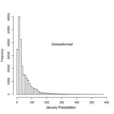
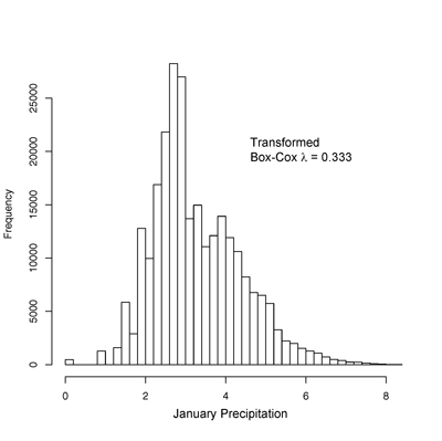
The histogram on the left below shows the distribution of January precipitation, while that on the right shows that for transformed January precipitation with lambda = 0.3333, (i.e. the commonly used “cube-root” transformation for precipitation).  For comparison, analogues were also calculated using untransformed variables.

Dissimilarity Measures

Two dissimilarity measures were used in this demonstration:  1) the widely used Euclidian-distance measure, and 2) the Mahalanobis distance, a statistical distance measure that takes into account the covariance among the variables.  Many of the variables (e.g. the monthly temperature variables, or GDD5 and MTWA), are highly correlated, and in a sense contribute redundant information to dissimilarity measures like the Euclidian distance.  The Mahalanobis distance can be thought of as an Euclidian-distance like measure, where the contributions of the individual variables to the distance are weighted by the elements of the inverse of the covariance matrix.  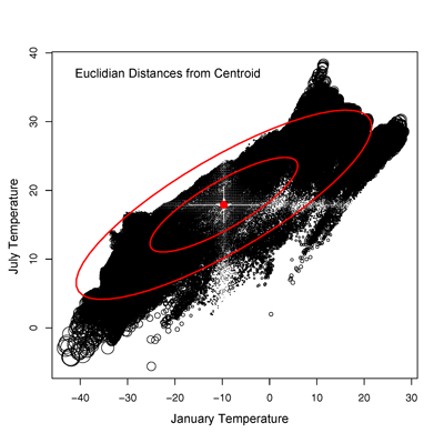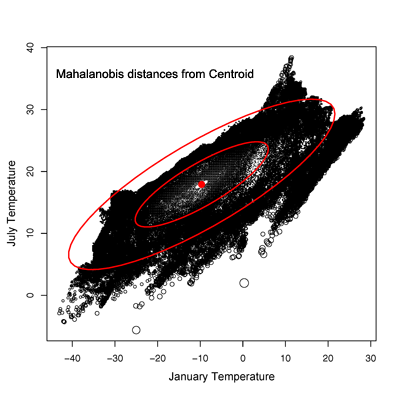The scatterplot on the left below shows the values of January and July temperature, with the Euclidian distance between each point and the centroid of the two variables indicated by the size of circle representing each point, while the scatterplot on the right shows the same thing for the Mahalanobis distances.  (Note; the obvious moiré pattern on the scatterplot on the left is created by the rasterization of the image.) The Mahalanobis distances can be thought of as the distance to the centroid measured across the isoprobability contours of a bivariate normal distribution fit to the data (shown in red).  Other dissimilarity measures could also be considered, like the Minkowski, or city-block distance.

Analogue Maps

An important issue is determining what constitutes an “analogue.”  One way of skirting this issue is to plot the analogues (dissimilarity values) on a continuous scale, but this would still require a user to choose some kind of intuitive threshold value to avoid distraction by low-analogue medium-dissimilarity value points.  The alternative of adopting some kind of single-value threshold is also unsatisfactory, because information on potential gradients in dissimilarities will be lost.  For this demonstration, a strict a and more liberal threshold was used in creating the maps.  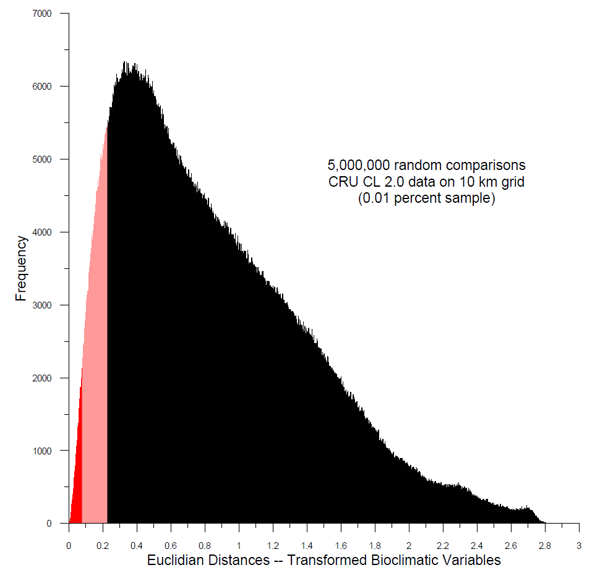The distribution of dissimilarity values created by comparing present-day observed (CRU) climate at  each point with those of all of the other points was estimated by 5 million random comparisons between the climate values at individual points (there are 48 x 10^9 total potential comparisons) for each analogue basis and transformation selection. The 1st  and 5th percentile values were selected as indicators of strong and weak (or less-strong) analogues.  The histogram below shows the random comparisons within the CRU 10-km data set for a set of bioclimatic variables (i.e. analogue-basis 4), with the 1st  and 5th percentile values shaded as dark and light red, respectively.  These values were used in creating the analogue maps.