bfh_python
A bordered Heegaard Floer computation package.
Overview and getting started
About bfh_python and this documentation
bfh_python is a package for doing computations of the Heegaard Floer homology group HF-hat of closed 3-manifolds, knot Floer homology of knots in 3-manifolds, and the bordered Heegaard Floer homology of 3-manifolds with boundary (preferably connected). It is written in Python, a widely-used and user-friendly interpreted programming language. It was written primarily by Bohua Zhan, with some contributions by Robert Lipshitz.
The mathematics underlying bfh_python is mostly in “Computing HF-hat by factoring mapping classes” (MathSciNet, article, arXiv) by Robert Lipshitz, Peter Ozsváth, and Dylan Thurston, and in Bohua Zhan’s Ph.D. thesis (MathSciNet, Princeton repository). Other citations are noted on the Mathematics page.
These pages document basic usage of bfh_python, as well as the structure and philosophy of the code itself, to help with extending it. Funding to support writing this documentation was provided by NSF Grant DMS-1810893. Any opinions, findings, and conclusions or recommendations expressed in this material are those of the author(s) and do not necessarily reflect the views of the National Science Foundation.
Getting started
To use bfh_python, you need:
- A Python interpreter or shell.
- The bfh_python package is available for download on github. New easier option! Nathan Dunfield has created a version you can install via PIP; pip installation instructions.
If you are familiar with Python and GitHub, please skip to the next section. Otherwise, some further advice follows.
Python interpreters (or shells)
I use the free version of PyCharm for working with Python, but it took a little effort to set up and if you just want to do a few computations, it is probably overkill. For Linux or a Mac, perhaps it is easiest to just install Sage, which comes with a nice Python shell. You can then work with bfh_python from either the Sage terminal or a Sage notebook. (The former is probably easier for following the instructions below.) For Windows, download the Python installer for Windows, install it, and run Python 3.8 from the start menu.
Downloading bfh_python
From bfh_python’s GitHub page, click the green “Clone or download” link and select “Download ZIP”.
Alternatively, you can clone the git repository: if you have git installed, from a terminal type git clone https://github.com/bzhan/bfh_python.git
Tutorials on basic usage
(Click on any image in the tutorial to enlarge.)
Computing the Heegaard Floer homology of a branched double cover
Perhaps the easiest application of the package is to compute the total dimension (over Z/2Z) of the Heegaard Floer homology of the branched double cover of the plat closure of a braid. For example, to compute the Heegaard Floer homology of the branched double cover of the (-2,3,5) pretzel
open a Python shell inside the folder (directory) containing bfh_python and type:
The output should look something like:
This is a bit confusing, but it means the result was a chain complex with one generator, called g1, and trivial differential. (The code already took homology.) Simpler is to ask about the length (dimension of a basis) of this complex:
gives output
That 1 means the result was 1-dimensional: we have an integer homology sphere L-space (in this case, the Poincaré homology sphere).
The syntax for the input is as follows. The name can be any string. The braid word uses i to denote σi and -i to denote σi-1. The bottom and top closures say how to cap off the braid on the two sides. If the braid has n endpoints they record the involution τ of {1,…,n} so that i and τ(i) are joined up.
Here’s the branched double cover of the torus knot T(3,5),
(The 5*[1,2] produces the list [1,2,1,2,1,2,1,2,1,2].) The result is a chain complex with one generator and trivial differential again (not a coincidence).
There’s actually a faster method for the last step, using Zhan’s notion of “local DA structures.” Instead of getHF() use:
The Heegaard Floer homology of some lens spaces and the Poincaré homology sphere
The following code computes the dimension of HF-hat of the lens space L(5,2):
The output of the final command should be 5, the dimension of HF-hat of L(5,2).
The steps in the code are:
- Import statements: tell Python to read in the pieces of the package that are needed for the computation.
- Let
Zbe the genus 1 pointed matched circle. (splitPMC(n)gives the genus n split pointed matched circle.) - Let solid_torus be a solid torus with the standard “infinity framing” (conventions are from “Computing HF-hat by factoring mapping classes”.)
- Let
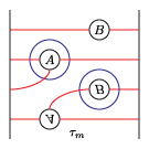
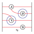
tau_mandtau_lbe the type DA bimodules associated to the two standard Dehn twists on the torus, which are the same as two arcslides in this case. (See the figure below.) - Tensor with these arcslide bimodules to change the framing on the solid torus to a (5,2) (or maybe (2,5)) framing.
- Create a zero-framed solid torus.
- Let
cfbe the chain complex of morphisms between the two. This is equivalent to gluing one of the solid tori to the mirror of the other. - Simplify
cfand compute the dimension of the result.
The bordered Heegaard diagrams for the solid tori at the different stages are:
(4) tau_m and tau_l, respectively: 

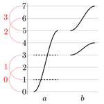
(5) solid_torus after tensoring each slide: 
You can inspect the type D structure for the framed solid tori. For example, to see the type D structures for the solid torus at the last stage, type:
(The first line replaces the very long names of generators with short ones. Try re-creating solid_torus and then typing solid_torus.generators without reindexing first and you’ll see what I mean.)
The output is:
This means: there are seven generators, g1 through g7. The differential of g3, for instance, is rho_2 times g2: rho_2 is the chord corresponding to a strand from point 1 to point 2. The differential of g5 is rho_123 times g_6; and so on.
In particular, this agrees with a by-hand computation for this bordered Heegaard diagram.
Important note
For arcslides, the input pointed matched circle (which becomes start_pmc in the Arcslide class) is on the left. The result of doing the specified arcslide to that pointed matched circle is on the right (and stored as end_pmc). When one tensors the arcslide to a type D structure, it is the right pointed matched circle end_pmc that gets glued to the type D structure. The new boundary is given by start_pmc. (Type D structures are left modules.) So, one often creates a list of arcslides from left to right, then reverses that list before tensoring it with a type D structure.
The Heegaard Floer homology of another branched double cover
We will compute the Heegaard Floer homology of the branched double cover of the following knot:
(I think this is L10n36.)
We could present this knot as a 4-bridge knot, but bfh_python is slow for wide knots. Instead, we’ll live with the cups in the middle.
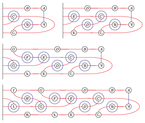
I get that the total dimension of HF-hat is 6. As a test, we can compute this the slow way, from the following bridge diagram:

(This is substantially slower on my computer.)
It is interesting to compare with Seed’s computation of Szabó’s geometric spectral sequence, in KnotKit. For this knot diagram, KnotKit finds the dimension of the E-infinity page is 12=(2)(6), as expected.
Some elements of the bordered algebra and the homology of the algebra
Code for working with the bordered algebras is in pmc.py. The main classes are:
PMC: represents pointed matched circlesStrandAlgebra: represents a bordered algebraStrandDiagram: represents a generator of a bordered algebraStrandAlgebraElement: an element of a strand algebra.
There are also some helper functions, like splitPMC, linearPMC, and antipodalPMC to generate particular pointed matched circles.
For example, the following code computes the generators
of the genus 2 pointed matched circle, their product, and the differential of each of them:
Here:
F2is the ground field, the field with two elements.idem_sizeis the number of pairs in an idempotent, from 0 to 2k for a genus k pointed matched circle.left_idemandright_idemare lists of which alpha-arcs are occupied (see the picture above). Each is a subset of {0,…,2k-1}. It is not necessary to specify bothleft_idemandright_idem.strandsis a list of the pairs of points in {0,…,4k-1} connected by strands.mult_oneindicates whether to quotient by the acyclic ideal of algebra elements with multiplicity >1 somewhere.
The output of multiplication or the differential is a StrandAlgebraElement. The element 0 is represented by E0. So, for example
is True. You can use pmc.pairid to find out which points on the pointed matched circles correspond to which matched pairs (for idempotents); for example, above, spmc.pairid[3] is 1.
There is a shorthand way to get strand diagrams from pmc.sd(); for example
both are True.
Here is code which computes the homology of alg:
The answer, 98, agrees with the literature.
Testing your copy of the package
The files ending “test.py” have code to test that the package is working. For example, “pmctest.py” has code to test “pmc.py” (which has classes for pointed matched circles and their algebras). To run one of these test files – pmctest.py, for instance – from the command line (not a Python shell) run:
To run all of the test files, run the script “testmod” or, have it display how fast the tests ran, run “testmodp”.
Warning
Some of the test code – particularly “braidtest.py” – takes a while to run.
Finding help inside the package
Many of the classes and functions in the package have “doc strings”, short explanations of how they work immediately after their declarations. For example, the Braid class in braid.py helpfully explains:
From inside a python shell, you can access these using the help command. For example:
Another source of help – and a big source of sample code – are the test files (see above).
Package limitations
Most of the package’s limitations come from limitations of bordered Heegaard Floer homology as currently constructed. In particular:
- The package only computes HF-hat, not HF-minus or other variants.
- All computations are over Z/2Z, the field with two elements.
- The package does not compute the absolute grading. It does compute the decomposition into spinc-structures and the relative gradings; see the Further Tutorials.
- The efficiency of the package is strongly related to the Heegaard genus; above Heegaard genus 5, computations are typically too slow to be useful, and in Heegaard genus 4 and 5, computations are somewhat slow.
There are other milder limitations, some of which would be easy to address. For example, there isn’t efficient code to check if two type D structures are homotopy equivalent, and there is no code to tensor together type DA bimodules.
Further documentation
The rest of this website has:
- A brief summary, with references, of the mathematics underlying bfh_python. This is aimed at someone familiar with Heegaard Floer homology but not with bordered Heegaard Floer homology. The summary tries to describe enough of the structure of the theory for one to understand how bfh_python’s components fit together, and what they can and cannot do.
- The structure of the bfh_python package. What the different classes encode and how they fit together.
- Further tutorials. A few more pieces of sample code, with brief explanations, exploring other features of bfh_python or reproducing computations from the literature.
Funding to support writing this documentation was provided by NSF Grant DMS-1810893. Any opinions, findings, and conclusions or recommendations expressed in this material are those of the author(s) and do not necessarily reflect the views of the National Science Foundation.
© 2019 - 2026 Robert Lipshitz lipshitz@uoregon.edu


