Chapter 7 Difference-in-differences
General setup
While sharing that the treatment effect will refer to the causal effect of a binary (0-1) variable on an outcome variable of scientific or policy interest difference-in-differences (DD) designs rely on a different assumption:
- Even where one might not be prepared to make the assumption that the treatment and control groups are the same in every respect apart from the treatment, it could be reasonable to make the assumption that in the absence of treatment the unobserved differences between treatment and control groups are the same over the period of analysis.
Where this is reasonable, one could use pre-treatment data on treatment and control groups to estimate the “normal” difference between treatment and control groups and then compare this to the difference after the receipt of treatment.
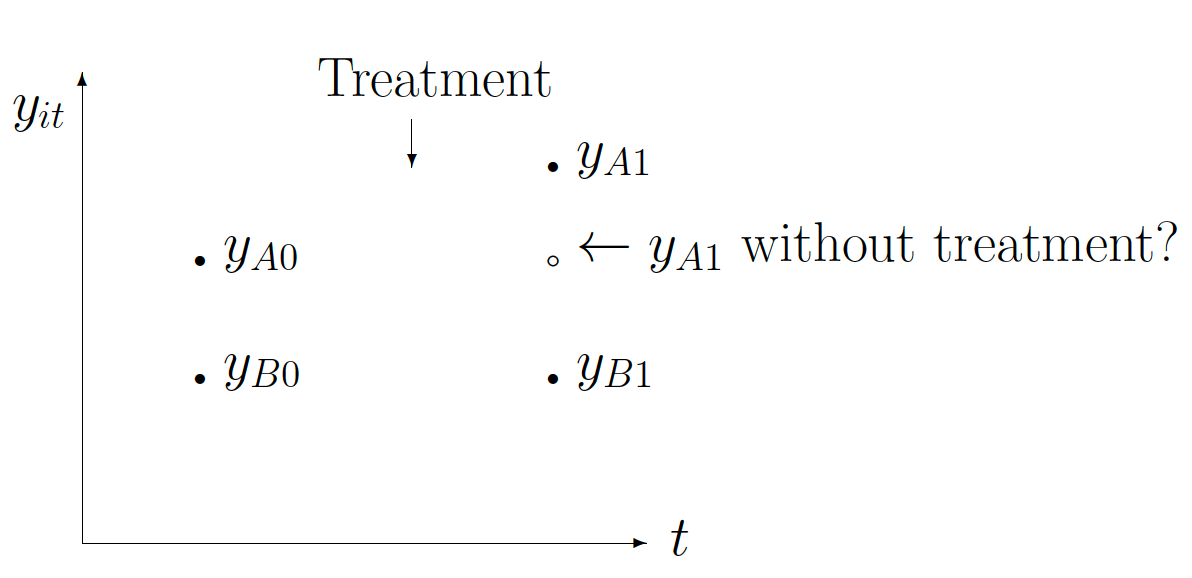
Consider using only data from the post-treatment period, measuring the “treatment effect” as the distance \(y_{A1}−y_{B1}\). This estimate is based on the assumption that the only reason for observing a difference in outcome between treatment and control group is the receipt of treatment. (Again, in an experimental setting this may well be successfully defended.)
In contrast, the DD estimator uses the “normal” difference between the treatment and control groups (i.e., the distance \(y_{A0} − y_{B0}\)) to facilitate the estimation of the treatment effect \((y_{A1}−y_{B1}) - (y_{A0}−y_{B0})\).
Note that the validity of this is based on the assumption that the “trend” in \(y\) is the same in both treatment and control groups throughout the period of analysis. If, for example, the trend was greater in the treatment group, the DD would attribute to treatment what is mere trending difference.
- With only two observations on \(t\), we can’t test this identifying assumption of the same trend in the absence of treatment.
- With more than two observations (of both treatment and control groups) one can (i.e., must) test whether pre-treatment trends differ between treatment and control groups. At the same time… this is not a test of the identifying assumption. (Hence… an assumption.)
Define \(\mu_{it}\) to be the mean of the outcome in group \(i\) at time \(t\). Define \(i=0\) for the control group and \(i=1\) for the treatment group. Define \(t=0\) to be a pre-treatment period and \(t=1\) to be the post-treatment period (though only the \(i=1\) group receives the treatment). The single-difference estimator simply uses the difference in post-treatment means between treatment and control groups as the estimate of the treatment effect (i.e., it uses an estimate of \(\mu_{11} - \mu_{01}\)). However, this assumes that the treatment and control groups have no other differences apart from the treatment—a very strong assumption with non-experimental data. A weaker assumption is that any differences in the change in means between treatment and control groups is the result of the treatment (i.e., to use \(\left(\mu_{11} - \mu_{01}\right) - \left(\mu_{10} - \mu_{00}\right)\), which is itself an estimate, as the estimate of the treatment effect—this is the difference-in-differences estimator).
How can one estimate this in practice? One way is to write the DD estimator as \(\left(\mu_{11} - \mu_{10}\right) - \left(\mu_{01} - \mu_{00}\right)\). Note that the first term is the change in outcome for the treatment group and the second term the change in outcome for the control group. Given these, one can simply estimate the model: \[\begin{equation} \Delta y_i = \beta_0 + \beta_1 X_i + \epsilon_i, \label{DDdeltay} \end{equation}\] where, \[\begin{equation} \Delta y_i = y_{i1} - y_{i0}. \end{equation}\]
Note that this is simply the differences estimator applied to differenced data, where \(X_i\) is an indicator variable taking the value 1 if the individual is in the treatment group and 0 if they are in the control group.
To implement the difference-in-differences estimator in the form above requires data on the same individuals in both the “pre” and “post” periods. But, it might be the case that the individuals observed in the two periods are different so that those in the pre-period who are in the treatment group are observed prior to treatment but we do not observe their outcome after the treatment. If we use \(t=0\) to denote the “pre-period” and \(t=1\) to denote the “post-period” and \(y_{it}\) to denote the outcome for individual \(i\) in period \(t\), then an alternative regression-based estimator (that just uses the level of the outcome variable) is given by the model:
\[\begin{equation} y_{it} = \beta_0 + \beta_1 X_{i} + \beta_2 T_{t} + \beta_3 X_i \cdot T_{t} + \epsilon_{it}, \label{DDy} \end{equation}\]where \(X_i\) is an indicator variable taking the value 1 if the individual is in the treatment group and 0 if in the control group, and \(T\) is an indicator variable taking the value 1 in the post-treatment period and 0 in the pre-treatment period. This is demonstrated quite explicitly in the table below.
| Treatment | Control | Difference | |
|---|---|---|---|
| Before | \(\beta_0 + \beta_1\) | \(\beta_0\) | \(\beta_1\) |
| After | \(\beta_0 + \beta_1 + \beta_2 + \beta_3\) | \(\beta_0 + \beta_2\) | \(\beta_1 + \beta_3\) |
| Difference | \(\beta_2 + \beta_3\) | \(\beta_2\) | \(\beta_3\) |
The DD estimator is going to be the OLS estimate of \(\beta_3\), the coefficient on the interaction between \(X_i\) and \(T_t\). Note that this is an indicator variable that takes the value one only for the treatment group in the post-treatment period.
Where one has repeated observations on the same individuals one can use either equation, on the same data—they will yield the same estimate of the treatment effect. However, the standard errors of that estimate will be different in the two cases.
You can include additional regressors in either formulation. Note, however, that if you think it is the level of some variable that has influence on the level of \(y\) then you should probably include the change in that variable as one of the other regressors if estimating the model in differenced form.
An example
There’s plenty of “marijuana-on-the-RHS” stuff being worked on, using medical and/or recreational legalization for identification. Let’s consider the first stage, though… the effect of legalization on marijuana use. Is it a problem if marijuana use is different in states that legalize?
- A better question? “When would it be a problem and when would it not be?” And, the answer depends on what inference statement one is tempted to make. We haven’t made any inference statements, so we cannot yet be wrong.

Suppose we were wanting to use a difference estimator. Is it a problem if marijuana use is different in states that legalize, and we want to attribute differences in use to having been treated? To legalization?
- Yes, of course. Pre-existing differences couldn’t possibly be due to treatment. And, if those differences continued into post treatment periods, we don’t have identification.
So… Suppose we were to use a difference-in-differences estimator. Is it a problem if marijuana use is different in states that legalize, and we want to attribute changes in those differences in use to legalization?
- Not at all. Our design “differences that out.” (That pre-treatment difference is the “differences” in “difference in differences.”)
What if marijuana use was increasing faster in treated states? (Could easily imagine that RML was endogenous to demand.) Would this be a problem?
- No clue. We haven’t made an inference statement yet.
If marijuana use was increasing more in treated states, and we wanted to attribute the difference in the level differences (across treatment nd control periods) to treatment?
- Yes, this would be a problem, as differential trends would lead to bias in the estimated change in relative levels pre and post treatment. (Is the direction of bias knowable?)
Ashenfelter (1978)
The assumptions necessary in DD analyses do not always hold so reasonably. In Ashenfelter (REStat 1978), the research question related to estimating the effect of government-sponsored training on earnings. The author took a sample of trainees under the Manpower Development and Training Act (MDTA) who started their training in the first three months of 1964. Their earnings were tracked both prior, during, and after training from social security records. A random sample of the working population was used as a comparison group. The average earnings for white males for the two groups in the years 1959-69 inclusive are as shown in this figure.
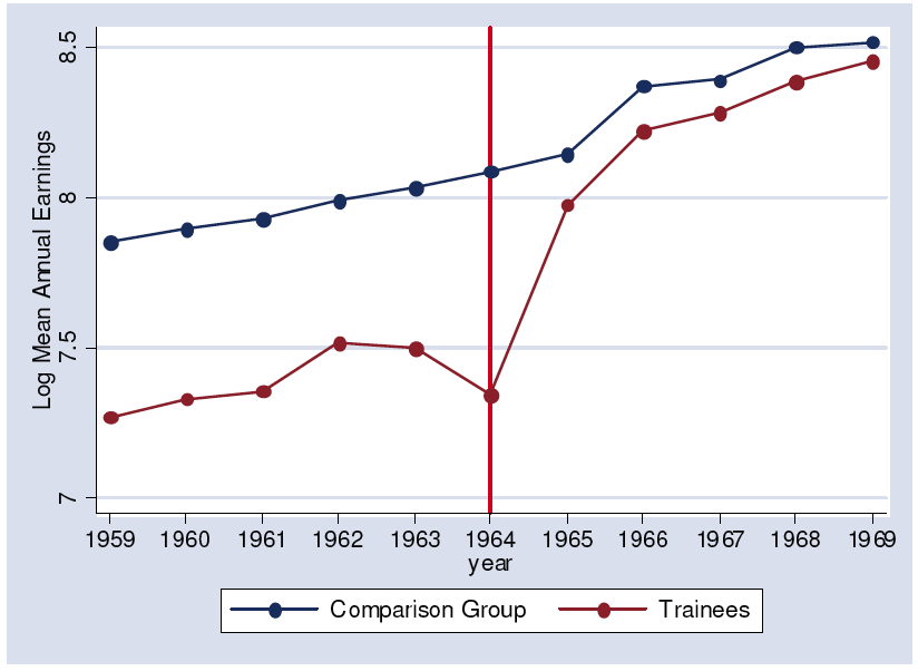
Figure 7.1: Figure: Dip among treated, as in Ashenfelter (REStat 1978)
There are several points worth noting:
- Earnings of the trainees in 1964 are very low because they were training and not working for much of this year—we should not pay much attention to this.
- The trainee and comparison groups are clearly different in some way unconnected to training as their earnings both pre- and post-training are different. This means that the difference estimator based on 1965 data would be very misleading as a measure of the impact of training on earnings. This suggests a difference-in-differences approach.
A simple-minded approach would use the data from 1963 and 1965 to give a difference-in-difference estimate of the effect of training on earnings. However, inspection of the associated time-series plots suggest that the earnings of the trainees were low not just in the training year, 1964, but also in the previous year, 1963. (Note that they are only slightly lower than 1962 earnings but the usual pattern is for earnings growth, leaving it quite a lot lower than what one might have expected to see.) This is what is now known as Ashenfelter’s Dip. The most likely explanation is that the trainees had a bad year that year (e.g., they lost a job) and it was this that caused them to enter training in 1964. Because trainees’ earnings are rather low in 1963, a simple difference-in-differences comparison of earnings in 1965 and 1963 is likely to overestimate the returns to training. (Ashenfelter describes a number of ways to deal with this problem—the point is that observations on multiple years can be used to shed light on whether the assumption underlying the use of difference-in-differences is a good one.)
DD with panel data
The above discussion of DD estimators implied only two observations on treatment and control groups. This is the most rudimentary form of panel data. While entire books are written about the analysis of panel data, sometimes giving the impression that the analysis of such data requires very different ideas and estimation technologies, the basics are not very different from standard regression.
Denote the number of individuals in the data set by \(N\) and the number of time periods over which we have information on the individual by \(T\). (Restrict our attention to balanced panels in which we have the same number of observations on every individual—the analysis of unbalanced panels in which we have more observations on some individuals than others is not much more difficult but the notation is messier.) Denote by \(y_{it}\) the outcome variable for individual \(i\) in period \(t\)—similarly define it \(x_{it}\).
In total we will have \(NT\) observations. One difference from normal cross-section data is that when we do asymptotics and take the number of observations to infinity, we can do this in a number of ways — \(N\) can go to infinity with \(T\) fixed, \(T\) can go to infinity with \(N\) fixed, or both \(N\) and \(T\) could go to infinity. It is most common to see the “large \(N\), fixed \(T\)” case because that is felt to be the best approximation to the situation in which researchers in microeconomics find themselves. But in other parts of the subject (macroeconomics, for example), it is common to be in a “fixed \(N\), large \(T\)” case for which the asymptotics can be very different.
A first approach to estimating models using panel data would be to ignore the panel nature of the data and simply estimate \[y_{it} = \beta' x_{it} + \epsilon_{it}.\]
OLS estimation of this will lead to a consistent estimate of \(\beta\) if \(E(\epsilon_{it} | x_{it})=0\).
However, unless STATA is told otherwise, the standard errors will be computed under the assumption that the \(\epsilon_{it}\) are all independent of each other, something that is very unlikely. For example, the outcome variable for the same individual is likely to be (strongly) correlated over time. There are a number of ways in which one might capture this idea—I will discuss one of them.
Introduce an individual specific component, and write \[y_{it} = \beta' x_{it} + \theta' D_i + \epsilon_{it},\] where \(\theta\) is an \(N\times1\) vector and \(D_i\) is a vector consisting of zeros everywhere except for a “1” in the \(i^{th}\) position. This equation will often be written more commonly as \[y_{it} = \beta' x_{it} + \theta_i + \epsilon_{it}.\]