Chapter 9 Instrumental variables

library(stargazer)

General discussion

To identify many (interesting) parameters requires attention to the fact that the variation in many of the variables whose effects are of interest may not be orthogonal to unobservable factors that jointly affect the outcomes studied. In determining the returns to schooling, for example, one cannot consider individuals to be randomly sorted across schooling levels. Thus, that more-schooled individuals have higher earnings may reflect the fact that more-able individuals prefer schooling or face lower schooling costs. Similarly, that fertility and female labor supply are negatively correlated may reflect variation in preferences for children and work in the population.

Some economists have used experiments that purposely randomize treatments to assess their effects in the presence of heterogeneity: negative income tax on labor supply; the effects of class size on test outcomes; or the effects of job-training programs on earnings.

These “man-made” experiments are subject to the criticisms that they lack generalizability and, most important, often do not adhere in implementation to the requirements of treatment randomness.

A common approach to identifying causal or treatment effects—one with a long history in economics—is to employ instrumental-variable techniques.

Not surprisingly, the assumptions made (inclusive of randomness) are subject to much skepticism.
Given the costs of carrying out and financing experiments with near-perfect random treatments, economists and other researchers often seek out sought “natural experiments.”
- changes (or spatial variation) in rules governing behavior, which are assumed to satisfy the randomness criterion
Many studies do not produce easily generalizable results about behavior because of the specific nature of the rule changes that are studied. The major problem with these studies, however, tends to be the assumption of randomness (which is often not credible).

In recent years, in recognition that “nature” can often provide almost perfect randomness with respect to important variables, economists have exploited naturally random events as instrumental variables. For example, several random outcomes that arise from biological and climate mechanisms have been used as instruments, including

twin births, human cloning (mono-zygotic twins), birth date, gender, and weather events.

These natural outcomes, which are plausibly random with respect to at least two of the major sources of heterogeneity in human populations (i.e., tastes and abilities) have been used to speak to such questions as

What are the returns to schooling and labor market experience?
How sensitive are consumption, savings, and labor supply to temporary and permanent changes in income?
How responsive is female labor-force participation to changes in fertility?

Instrumental variable (IV) methods deal with the endogeneity of a regressor within a linear-regression framework. The instrument itself, or the exclusion restriction, is a variable that affects the endogenous variable but does not affect the outcome variable other than through its effect on the endogenous variable.

Instrumental-variable methods are also used in measurement-error contexts. In the last ten years, there has been a revolution in the interpretation of IV estimates as the literature has begun to investigate IVs in contexts where the effect of the endogenous variable varies across units in ways that may or may not be related to the instrument.

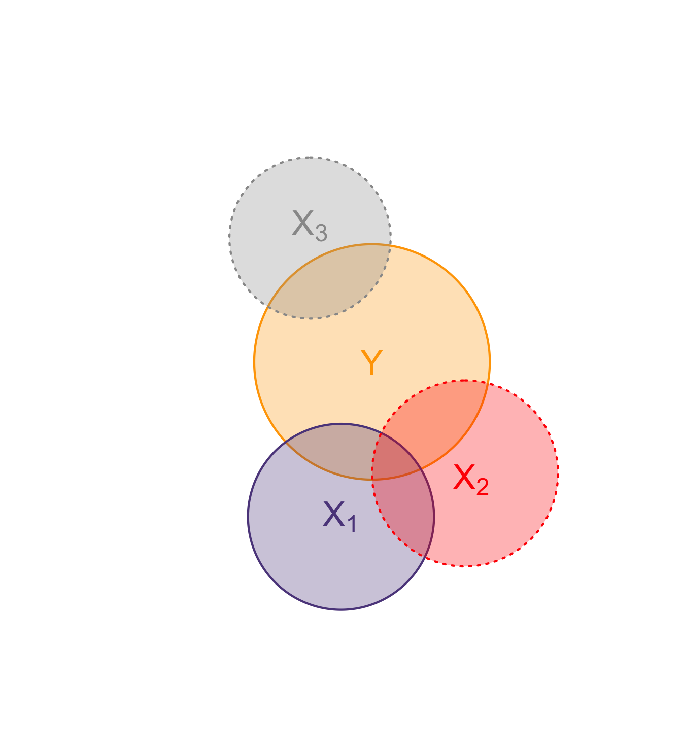
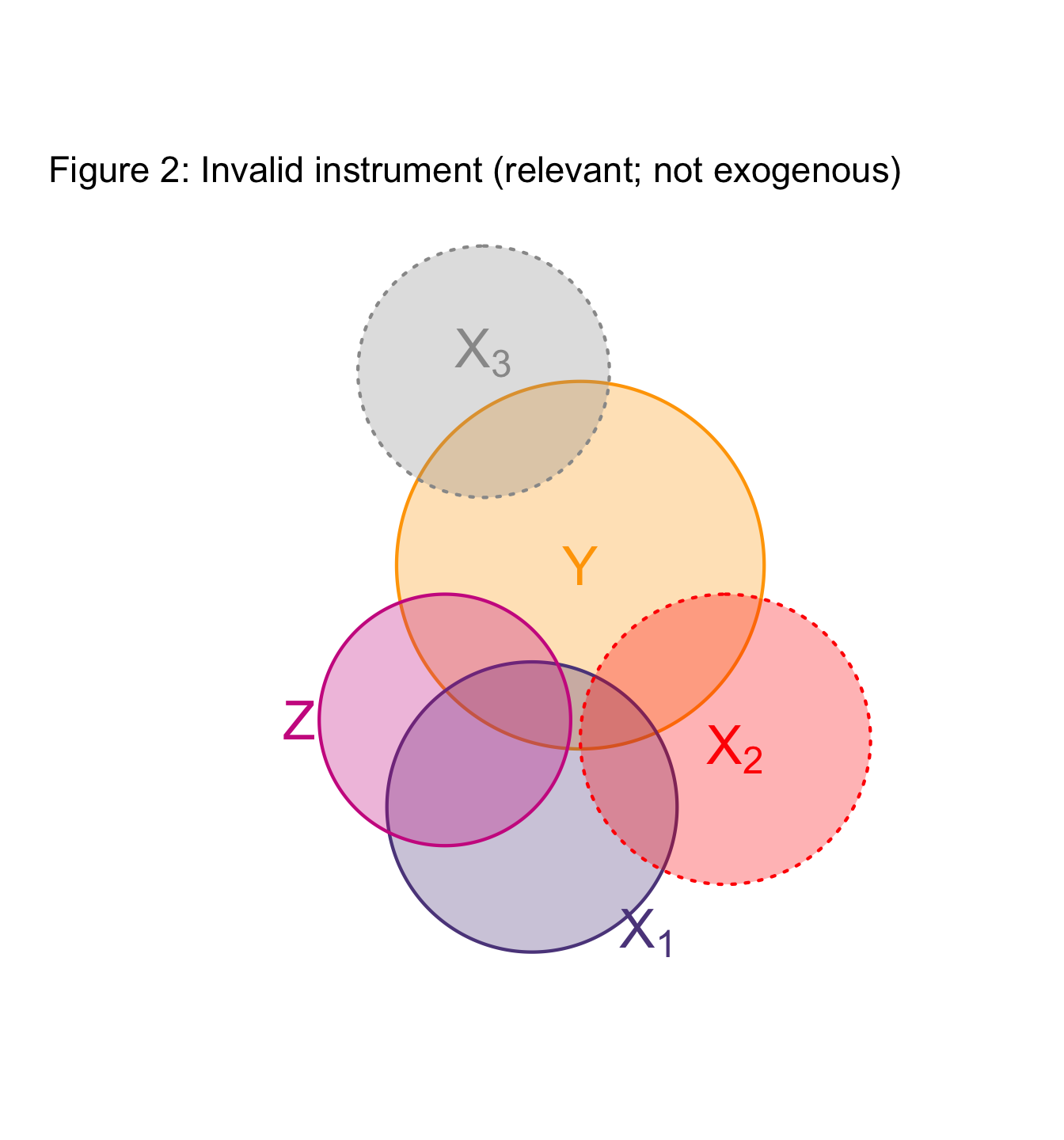
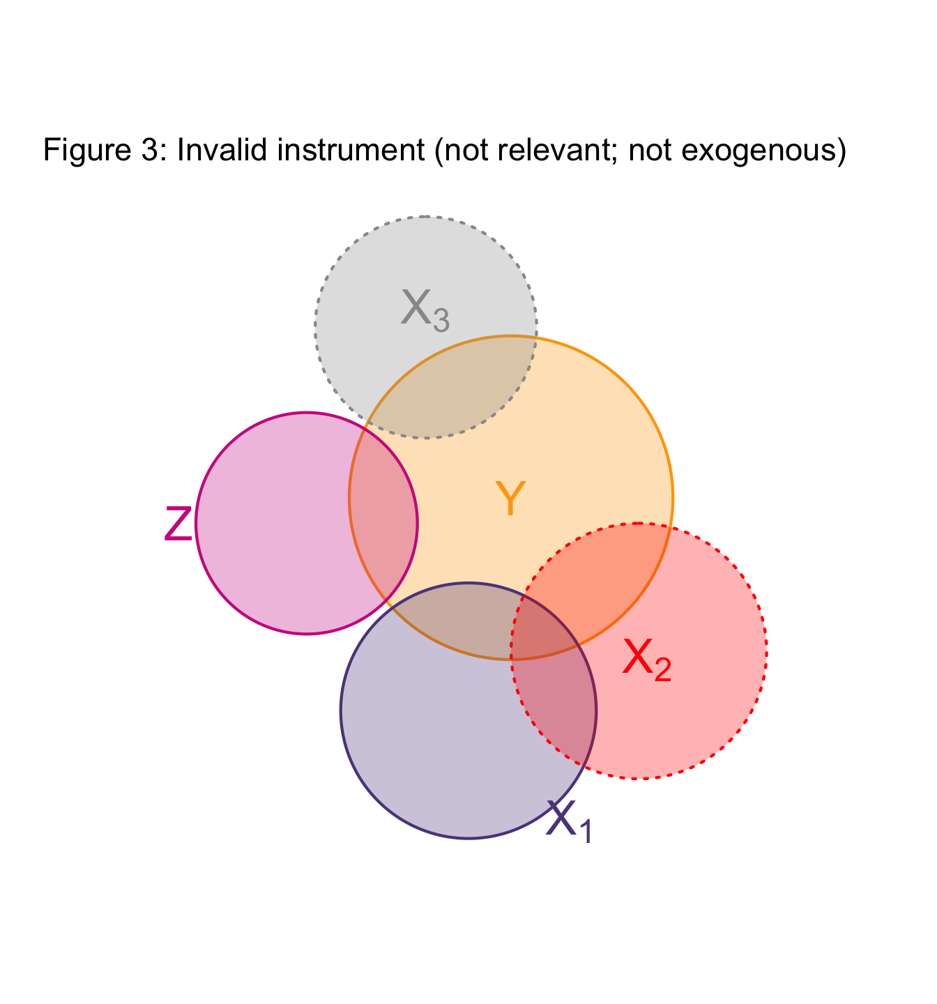
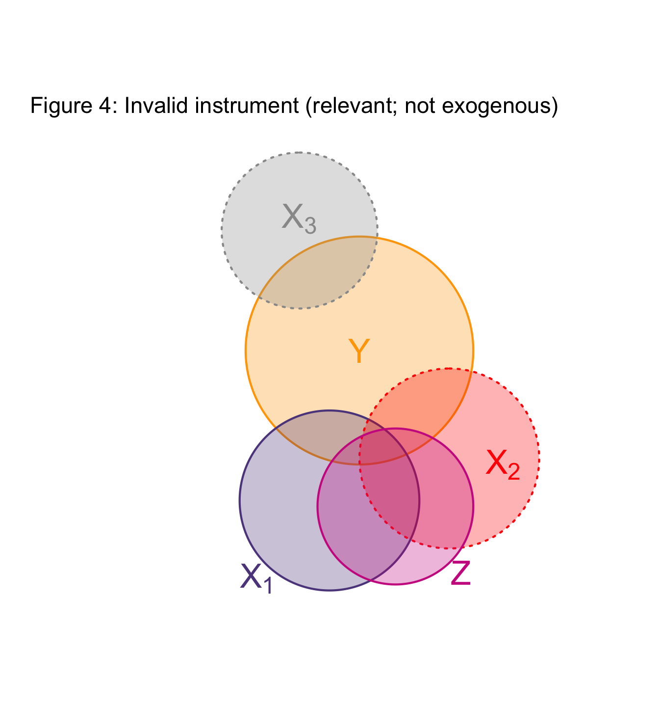
IV in pictures

Again with an abstraction… but a useful one

In these figures (Venn diagrams)

Each circle illustrates a variable.
Overlap gives the share of correlatation between two variables.
Dotted borders denote omitted variables.

Example: Project Star

By way of example, consider Tennessee’s Project Star—a random-assignment evaluation of changing the size of primary school class sizes from 24 students to 18 students. Are smaller classes better? (The outcome variable of interest is test scores.)

Define the following notation:

$Y$ = average test score for class “$i$”
$X_i \in \{18, 24\}$ is the number of students in class “$i$”
$Z_i \in \{0, 1\}$ equals 1 for a small class (the treatment) and 0 for a large class (the control)

The reduced-form model gives the direct effect of being assigned to the treatment group on outcomes:

\[Y_i = \Pi_0 + \Pi_1 Z_i + v_i,\]

where $\Pi_1$ is of direct policy interest. However, we are also interested in the structural parameter, namely the derivative of test scores with respect to class size. That parameter appears in the structural equation:

\[Y_i = \beta_0 + \beta_1 X_i + \epsilon_i,\]

where $\beta_1 = \partial Y / \partial X$. In terms of the notation above, the coefficient from the reduced-form model may be written as

\[\Pi_1 = \frac{\partial X}{\partial Z}\frac{\partial Y}{\partial X}.\]

Given random assignment, one might think about estimating the structural model directly. However, practical concerns can often intervene. For example, in this case, random assignment was defeated at the margin by some parents. To the extent this occurred, one would actually want to estimate the structural parameter of interest indirectly using IV.

We can obtain the first component by estimating the first-stage model,

\[X_i = \theta_0 + \theta_1 Z_i + u_i.\]

If random assignment worked perfectly, then $\hat{\theta}_1$ would equal $-6$. However, given the empirical problems identified, $\hat{\theta}_1$ will actually lie in $[-6,0]$.

The IV estimate is then given by the ratio of the reduced-form estimate from the outcome equation to the coefficient from the first stage, or

\[\beta_1 = \frac{\partial Y}{\partial X}=\frac{{\hat \Pi_1}}{{\hat \theta_1}}.\]

This estimate is consistent, despite the partial disruption of random assignment. However, if disruptions of random assignment are not random with respect to expected test scores, the error term in that equation will be correlated with the class size variable. If this is the case, the estimate based on direct estimation of the structural equation would not be consistent.

The just-identified case

Suppose that we have non-experimental data and just one endogenous covariate, $x$. Thus, we have that

\[y_i = \beta_0 + \beta_1 x_i + \epsilon_i,\]

where $cov(x_i,\epsilon_i) \ne 0$. Because of the endogeneity problem, we cannot impose the second of the OLS orthogonality conditions (which is equivalent to saying the second of the OLS first-order conditions). Suppose instead that we have an instrument, a variable $z_i$, such that $cov(z_i,\epsilon_i) = 0$ and $cov(z_i,x_i) \ne 0$.

(Note that in the general case with more covariates, all that is required is that the covariance of $z_i$ and $\epsilon_i$ conditional on $x_i$ equal zero.)

Deriving the estimator

With such a variable, we can utilize an alternative orthogonality condition based on $cov(z_i,\epsilon_i)=0$ to derive an estimator. To see this, note that the covariance condition implies that

\[z_i(y_i - \beta_0 - \beta_1x_i ) = 0\]

This is the same as the analogous OLS first-order condition, but with $z_i$ in place of $x_i$.

Proceeding with the usual derivation but with this replacement leads to

\[{\hat \beta_{IV}}=\frac{\sum_{i=1}^{n}(y_i-{\bar y})(z_i-{\bar z})}{\sum_{i=1}^{n}(x_i-{\bar x})(z_i-{\bar z})}\]

Using the notation from the Project Star example, this falls out easily. Recall that

\[{\hat \theta_{1}}=\frac{\sum_{i=1}^{n}(z_i-{\bar z})(x_i-{\bar x})}{\sum_{i=1}^{n}(z_i-{\bar z})^2}\]

and that

\[{\hat \Pi_{1}}=\frac{\sum_{i=1}^{n}(z_i-{\bar z})(y_i-{\bar y})}{\sum_{i=1}^{n}(z_i-{\bar z})^2}.\]

As in the Project Star example, the ratio then gives

\[{\hat \beta_1} = \frac{{\hat \Pi_1}}{{\hat \theta_1}}\]

The Wald estimator

A useful special case occurs when both the endogenous variable and the instrument are binary. In this case, the IV formula reduces to a simple form called the Wald estimator.

Consider the reduced-form outcome model. In the case of a binary instrument, the coefficient on the instrument is simply the mean difference in outcomes between units with the instrument equal to one and units with the instrument equal to zero. In notation, the first-stage coefficient equals

\[{\hat \Pi_{1}}={\hat E}(Y | Z = 1) - {\hat E}(Y | Z = 0)\]

where the expectations are estimated by sample means.

Similarly, the first-stage regression of the endogenous variable on the instrument is a linear-probability model in this case. The coefficient on the instrument is just the mean difference in the probability that the endogenous dummy variable equals one for units with the instrument equal to one and units with the instrument equal to zero. In notation, the first stage coefficient equals

\[{\hat \theta_{1}}={\hat Pr}(D=1 | Z = 1) - {\hat Pr}(D =1 | Z =0)\]

where $D$ is the endogenous binary variable.

Combining the two estimates using the formula above gives the Wald estimator

\[{\hat \Delta_{IV}}=\frac{\Pi_1}{\theta_1}=\frac{E(Y | Z=1)-E(Y | Z=0)}{Pr(D=1 | Z = 1) - Pr(D=1 | Z = 0)}.\]

The intuition here is that the denominator serves to scale up the mean difference in outcomes to account for the fact that the change in the instrument changes the status for some but not all individuals.

Another example (distance as IV)

Consider a simple example, which will use distance from a training center as an instrument to measuring the effect of training on some outcome $Y$.

To begin, consider a training center located in one town but which serves the residents of two towns. Those in the same town as the training center have only a short distance to travel for training, while those in the other town have a long distance to travel.

Suppose that the marginal effect of training on those who undertake the training is $\Delta = \$10$, and that the outcome in the absence of training is $Y_0 = \$100$.
The tuition for the training course is $5. Everyone pays this.
For those in the near town, there are no travel costs. For those in the far town, the travel cost depends on whether the individual has a car or not. For those with a car, the cost is essentially zero. For those without a car, the cost is $12.
- Assume that half of the eligible persons have a car and that there are 200 eligible persons in each town.
- Assume that everyone knows both their costs and benefits associated with training, and participates only when the benefits exceed the costs.

Let $Z = 1$ denote residence in the near town and $Z = 0$ denote residence in the far town. Let $D =1$ denote participation in training and $D = 0$ denote non-participation.

Using our standard notation, let

\[Pr(D=1|Z=1)=1.0,\]

and,

\[Pr(D=1|Z=0)=0.5.\]

Thus, there is a difference in participation probabilities depending on whether one resides in the near town or the far town. That is to say that our instrument is correlated with the endogenous variable. At the same time, by construction the instrument is not correlated with the untreated outcome (which is a constant in this example). Thus, the instrument meets the two criteria for validity.

The IV estimator in this simple case is given by:

\[{\hat \Delta_{IV}}=\frac{E(Y | Z=1)-E(Y | Z=0)}{Pr(D=1 | Z = 1) - Pr(D=1 | Z = 0)}.\] The denominator serves to scale up the mean difference in outcomes to account for the fact that the change in the instrument changes the status for some but not all individuals.

In this example,

\[E(Y | Z = 1) = Y_0 + \Delta Pr(D = 1 | Z = 1) = 100 +10(1.0) = \$110\]

and

\[E(Y | Z = 0) = Y + \Delta Pr(D = 1 | Z = 0) = 100 +10(0.5) = \$105.\]

As expected, then,

\[{\hat \Delta_{IV}}=\frac{110 - 105}{1.0 - 0.5}=\frac{5}{0.5}=\$10.\]

Note: Adopting an ordinary least squares approach alone (e.g., some $Y_i = \beta_0 + \beta_1 Z_i + \epsilon_i$), would yield an estimated coefficient on $Z_i$ of $\beta_1 = 5$.

Running IV models

IV in STATA

The command in STATA estimates models using instrumental variables or two-stage least squares. (Note: ivreg is an out-of-date command as of Stata 10. ivreg was been replaced with the ivregress command.) The format of the command is

ivregress <depvar> <exogenous x> (<endogenous x> = <excluded IVs>)

Thus, to estimate

\[y_i = \beta_0 + \beta_1x_{1i}+ \beta_2x_{2i}+ \beta_3x_{3i}+u_i,\]

where $x_3$ is endogenous and $z$ is an instrument for $x_3$, one would code

ivregress y x1 x2 (x3 = z)

The first option to the ivreg command causes STATA to display the results of both the first stage and second stage regressions. (Note, ivregress2 provides a fast and easy way to export both the first-stage and the second-stage results similar to ivregress, on which it is based.)

IV in R

library(AER)
# general form: 
ivreg(formula, instruments, data, etc)
#or
ivreg(y ~ <exogenous x> + <endogenous x> | . - <endogenous x> + <excluded IVs>, data = df)
# for example:
ivreg(y ~ x + d | x + z, data = df)
# or, put differently
ivreg(y ~ x + d | .-d + z, data = df)

Note: Endogenous variables can only appear before the vertical line; instruments can only appear after the vertical line; exogenous regressors that are not instruments must appear both before and after the vertical line.

Thus, to estimate

\[y_i = \beta_0 + \beta_1x_{1i}+ \beta_2x_{2i}+ \beta_3x_{3i}+u_i,\]

where $x_3$ is endogenous and $z$ is an instrument for $x_3$, one would code

ivreg(y ~ x1 + x2 + x3 | .-x3 + z)

Testing exogeneity

It can often be useful to test whether or not a potentially endogenous variable actually is endogenous. In the literature you will occasionally see papers that test the null hypothesis of exogeneity of the potentially endogenous variable. If this null is not rejected, the analysis will proceed under the assumption of exogeneity (and run OLS). If not, the analysis will undoubtedly proceed to undertake some sort of IV strategy.

This standard test compares the OLS and 2SLS estimates. Under the null (that the potentially endogenous variable is actually exogenous) these two estimates differ only due to sampling error. In contrast, under the alternative hypothesis (that the variable is actually endogenous) they should differ because the 2SLS estimator is consistent under the alternative (while OLS is not).

There are a number of different ways to perform this test. Two of the most common are as follows.

Method 1: Using first-stage regression residuals

This method is quite straightforward. It consists of taking the residuals from the first-stage estimation and including them in the second stage, along side the endogenous variable.

In notation, the first stage is given by

\[X_i=Z_i\gamma +v_i,\]

and the estimated residuals are given by

\[{\hat v_i} =X_i -Z_i{\hat \gamma}.\]

The second stage for the test is given by

\[Y_i=X_i\beta +{\hat v_i}\beta_v+u_i.\]

The test is, quite simply, the standard $t$-test of the null that the coefficient on the first-stage residuals equals zero. In notation, the null is given by

\[H_0:\beta_v = 0.\]

The intuition behind the test is that under the null of exogeneity, the residuals from the first stage are just noise, and so should have no predictive power in the second stage (and a coefficient of zero). In contrast, under the alternative hypothesis of endogeneity, the first-stage residuals represent the “bad” variation in the endogenous variable – the part that is correlated with the error term in the outcome equation – just as they do in the control-function version of the 2SLS estimator. In this case, their coefficient should be non-zero.

This test is easily generalized to the case of multiple endogenous variables. In this case, there is a vector of first-stage residuals – one for each of the endogenous variables – and the test takes the form of an $F$-test of the null that all of the coefficients on the estimated residuals equal zero.

Method 2: A $t$-test on the coefficient of interest

The second method focuses solely on the coefficient of interest, estimated using OLS and IV. )Typically the coefficient of interest is the coefficient on the endogenous variable.)

Call the coefficient of interest ${\hat \beta_k}$. The test then consists of examining the statistic

\[\frac{{\hat \beta_{k,2SLS}}-{\hat \beta_{k,OLS}}}{\sqrt{se({\hat \beta_{k,2SLS}})^2-se({\hat \beta_{k,OLS}})^2}},\] which has an asymptotic $t$ distribution. (The denominator is the standard error of the numerator under the null.)

The intuition here is that under the null, the coefficients differ only due to sampling error. The 2SLS estimator is inefficient, and so has a higher asymptotic variance, because it uses a less-efficient instrument for the endogenous variable under the null. Under the null of exogeneity, the efficient instrument for the potentially endogenous variable is the variable itself.

Issues with the variance of the difference: In practice, the estimated variance of the difference will sometimes not be positive definite; the ordering is asymptotic and may not hold in particular finite samples. This is one reason to prefer the regression-based tests. In this situation, STATA reports an error message and takes a generalized inverse so that a positive value results.

Other remarks: In Cambridge, Massachusetts, this is called the Hausman test. In Chicago, it is called the Durbin-Wu-Hausman test. Using all three names is probably the risk-averse choice; another alternative is to simply refer to it as the “standard exogeneity test.”

The null here is exogeneity. Thus, the test is, in the usual classical statistical sense, being conservative about concluding endogeneity. If theory (or even common sense) or evidence from other studies suggests endogeneity, this may suffice to proceed with 2SLS regardless of the results of the test.

Of course, such tests assume that you have a valid instrument, which can be a strong assumption in many cases. The implication of this is that if you fail to reject the null, it may be because the instrument itself is invalid, rather than because the variable in question is exogenous.

The discussions in Greene’s Econometric Analysis and in Wooldridge’s Econometric Analysis of Cross Section and Panel Data emphasize different issues associated with the test. The Greene discussion presents a Wald-test version of the $t$-test reported here. The test statistic in that test is essentially the $t$-test test statistic squared. The resulting test statistic has a $\chi^2$ distribution. Greene also presents an alternative regression-based version of the test due to Wu (Econometrica 1973). This version of the test includes the predicted values of the endogenous variables in the outcome equation along with the original $X$. The test consists of an $F$ test of the joint null that the coefficients on all of the predicted values equal zero. The intuition is that under the null the differences between the predicted values and the original values are only noise and so should not be related to the dependent variable.

The bottom line: if there is a reason to expect endogeneity but the test fails, it is nice to report both the OLS and IV estimates and the test results, and interpret the findings from the analysis accordingly.

Durbin-Wu-Hausman test in STATA

Before continuing, note that the D-W-H test is in fact far more general. The basic idea of comparing two estimates, one that is consistent both under the null and the alternative and one that is consistent only under the null, can be applied in many econometric contexts.

To implement the test in STATA do the following:

ivregress y x1 (x2 = z1)

where $y$ denotes the dependent variable, $x_1$ denotes the exogenous variables included in the outcome equation, $x_2$ denotes the endogenous variables included in the outcome equation and $z_1$ denotes the excluded instruments.

Next, do:

estimates save ivname

This tells STATA to save the IV results for later comparison with the OLS results. Then generate the OLS results by

reg y x1 x2

Finally, have STATA compare the OLS and IV results and do the Hausman test by using the hausman command a second time.

estimates save olsname
hausman ivname olsname, constant sigmamore

where ivname and olsname are the names that you give to the saved IV and OLS estimates, respectively. STATA uses the second version of the test, generalized to matrices.

Testing over-identifying restrictions

In some cases, you may have more candidate instruments than you do endogenous variables. In this case, because you only need as many instruments as there are endogenous variables for identification, there are over-identifying restrictions that can be tested. These restrictions consist of the exogeneity of the ``extra" instruments.

The intuition behind the test is to compare 2SLS estimates obtained using all of the instruments with those using just a necessary subset of the available instruments.

As this test is computationally burdensome, Wooldridge recommends a simple regression-based alternative. * In this alternative test, the 2SLS residuals from using all of the candidate instruments are regressed on all of the exogenous variables. Under the null that all of the instruments are valid, this regression should have a population $R^2$ value of zero. Under the alternative, the population $R^2$ is non-zero because some of the instruments are correlated with the error term, which is estimated by the 2SLS residuals.

Doing the regression-based test in STATA uses standard commands. Doing the original Hausman version of the test in STATA uses the same general structure as the exogeneity test. The sequence of commands is:

ivregress y x1 (x2 = z1)

estimates save ivconsist

This tells STATA to save the first set of IV results for later comparison (with the second set of IV results). Then, generate the second set of IV results by

ivregress y x1 (x2 = z1 z2)
estimates save iveffic

where $z_2$ denotes the instruments whose validity differs between the null and the alternative.

Finally, have STATA compare the two sets of IV estimates via the Hausman test by using the hausman command a second time.

ivregress y x1 (x2 = z1)
hausman ivconsist iveffic, constant sigmamore

where ivconsist and iveffic are just names given to the saved estimates from the consistent and efficient models, respectively.

There is also an .ado command (i.e., overid) that does the regression version of the test described above (and in Wooldrige) in one step, immediately following the estimation of the ivreg command.

Simulating IV (in R)

Suppose we wish to estimate $y=a+bx+cd+e$, where $y$ is to be explained, and $a$, $b$, and $c$ are the coefficients we want to estimate. $x$ is the control variable and $d$ is the treatment variable. We are particularly interested in the impact of our treatment $d$ on $y$.

First, let’s generate the data. Assume the the correlation matrix between $x$, $d$, $z$ (the instrumental variable for $d$), and $e$ is as follows:

R <-matrix(cbind(1,0.001,0.002,0.001,
                0.001,1,0.7,0.3,
                0.002,0.7,1,0.001,
                0.001,0.3,0.001,1),nrow=4)
rownames(R)<-colnames(R)<-c("x","d","z","e")
R

##       x     d     z     e
## x 1.000 0.001 0.002 0.001
## d 0.001 1.000 0.700 0.300
## z 0.002 0.700 1.000 0.001
## e 0.001 0.300 0.001 1.000

Specifically, note that $cor(d,e)=0.3$, which is us introducing that $d$ is endogeneous. $cor(d,z)=0.7$ implies that $z$ is a strong instrumental variable for $d$, while $cor(z,e)=0.001$ implies that $z$ might well satisfy the exclusion restriction (in that it only affects $y$ through $d$).

Now, let’s generate data for $x$, $d$, $z$, and $e$, with the specified correlation.

U = t(chol(R))
nvars = dim(U)[1]
numobs = 1000
set.seed(1)
random.normal = matrix(rnorm(nvars*numobs,0,1), nrow=nvars, ncol=numobs);
X = U %*% random.normal
newX = t(X)
data = as.data.frame(newX)
attach(data)
cor(data)

##             x          d            z           e
## x  1.00000000 0.00668391 -0.012319595 0.016239235
## d  0.00668391 1.00000000  0.680741763 0.312192680
## z -0.01231960 0.68074176  1.000000000 0.006322354
## e  0.01623923 0.31219268  0.006322354 1.000000000

Now let’s specify the true data-generating process that explains variation in $y$

y <- 10 + 1 * data$x + 1 * data$d + data$e

OLS

If we use $x$ and $d$ to explain $y$, ignoring the true relationship, retrieving a coefficient on $d$ other than 1 evidences bias.

ols<-lm(y ~ x + d, data)
summary(ols)

## 
## Call:
## lm(formula = y ~ x + d, data = data)
## 
## Residuals:
##     Min      1Q  Median      3Q     Max 
## -3.2395 -0.5952 -0.0308  0.6617  2.7592 
## 
## Coefficients:
##             Estimate Std. Error t value Pr(>|t|)    
## (Intercept)  9.99495    0.03105  321.89   <2e-16 ***
## x            1.01408    0.02992   33.89   <2e-16 ***
## d            1.31356    0.03023   43.46   <2e-16 ***
## ---
## Signif. codes:  0 '***' 0.001 '**' 0.01 '*' 0.05 '.' 0.1 ' ' 1
## 
## Residual standard error: 0.9817 on 997 degrees of freedom
## Multiple R-squared:  0.7541, Adjusted R-squared:  0.7536 
## F-statistic:  1528 on 2 and 997 DF,  p-value: < 2.2e-16

The OLS-estimated coefficient on $d$ is $1.31 \ne 1$.

2SLS

Now, let’s estimate the relationship with $z$ as the instrumental variable for $d$.

Stage 1: regress $d$ on $x$ and $z$, and save the fitted value for $d$ as d.hat

tsls1 <- lm(d ~ x + z, data)
data$d.hat <- fitted.values(tsls1)
#summ(tsls1, robust="HC1", confint=TRUE, digits=3)
summary(tsls1)

## 
## Call:
## lm(formula = d ~ x + z, data = data)
## 
## Residuals:
##      Min       1Q   Median       3Q      Max 
## -2.59344 -0.52572  0.04978  0.53115  2.01555 
## 
## Coefficients:
##             Estimate Std. Error t value Pr(>|t|)    
## (Intercept) -0.01048    0.02383   -0.44    0.660    
## x            0.01492    0.02296    0.65    0.516    
## z            0.68594    0.02337   29.36   <2e-16 ***
## ---
## Signif. codes:  0 '***' 0.001 '**' 0.01 '*' 0.05 '.' 0.1 ' ' 1
## 
## Residual standard error: 0.7534 on 997 degrees of freedom
## Multiple R-squared:  0.4636, Adjusted R-squared:  0.4626 
## F-statistic: 430.9 on 2 and 997 DF,  p-value: < 2.2e-16

Stage 2: regress $y$ on $x$ and d.hat

tsls2 <- lm(y ~ x + d.hat, data)
#summ(tsls2, robust="HC1", confint=TRUE, digits=3) 
summary(tsls2)

## 
## Call:
## lm(formula = y ~ x + d.hat, data = data)
## 
## Residuals:
##     Min      1Q  Median      3Q     Max 
## -4.4531 -1.0333  0.0228  1.0657  4.0104 
## 
## Coefficients:
##             Estimate Std. Error t value Pr(>|t|)    
## (Intercept)  9.99507    0.04786  208.85   <2e-16 ***
## x            1.01609    0.04612   22.03   <2e-16 ***
## d.hat        1.00963    0.06842   14.76   <2e-16 ***
## ---
## Signif. codes:  0 '***' 0.001 '**' 0.01 '*' 0.05 '.' 0.1 ' ' 1
## 
## Residual standard error: 1.513 on 997 degrees of freedom
## Multiple R-squared:  0.4158, Adjusted R-squared:  0.4146 
## F-statistic: 354.8 on 2 and 997 DF,  p-value: < 2.2e-16

In summary

The true value of the coefficient on $d$: 1
The OLS estimate of the coefficient on $d$: 1.314
The 2SLS estimate of the coefficient on $d$: 1.010

If the treatment variable is endogenous, an instrumental variable for the treatment variable retrieves the causal parameter, subject to its exclusion.

Note that, in the above, standard errors do not account for d.hta itself being an estimate.

Each of the elements in the population variance can be estimated from a random sample. The estimated variance is then, \[var(\hat \beta) = \frac{\sigma^2}{SST_xR^2_{x,z}},\] where $\sigma^2 = SSR$ from the IV divided by the df, and $SST_{x,z}$ is the sample variance in $x$, and the $R^2$ is from the first-stage regression (of $x$ on $z$).
- The standard errors is just the square root of this
SE in the IV case differs from OLS only in the $R^2$ from regressing $x$ on $z$.
- Since $R^2<1$, IV standard errors are larger
However, IV is consistent, while OLS is inconsistent when $cov(x,u)\ne0$.
Notice that the stronger the correlation between $z$ and $x$, the smaller are the IV standard errors.

Correct SE estimates in 2SLS (in R)

R has two instrumental-variables functions: tsls() in sem, and ivreg() in AER. Both have similar input formats, both use two-stage least squares to estimate their final equation, and both adjust the standard error of the final parameter estimates in a consistent fashion.

library(AER)

## Loading required package: car

## Loading required package: carData

## 
## Attaching package: 'car'

## The following object is masked from 'package:dplyr':
## 
##     recode

## The following object is masked from 'package:purrr':
## 
##     some

## Loading required package: lmtest

## Loading required package: zoo

## 
## Attaching package: 'zoo'

## The following objects are masked from 'package:base':
## 
##     as.Date, as.Date.numeric

## Loading required package: sandwich

## Loading required package: survival

ivreg.model <- ivreg(y ~ x + d | .- d + z, data = data)
summary(ivreg.model)

## 
## Call:
## ivreg(formula = y ~ x + d | . - d + z, data = data)
## 
## Residuals:
##       Min        1Q    Median        3Q       Max 
## -3.633059 -0.662849 -0.009458  0.721780  2.917705 
## 
## Coefficients:
##             Estimate Std. Error t value Pr(>|t|)    
## (Intercept)  9.99507    0.03259  306.71   <2e-16 ***
## x            1.01609    0.03141   32.35   <2e-16 ***
## d            1.00963    0.04659   21.67   <2e-16 ***
## ---
## Signif. codes:  0 '***' 0.001 '**' 0.01 '*' 0.05 '.' 0.1 ' ' 1
## 
## Residual standard error: 1.03 on 997 degrees of freedom
## Multiple R-Squared: 0.7291,  Adjusted R-squared: 0.7286 
## Wald test: 765.1 on 2 and 997 DF,  p-value: < 2.2e-16

Card (1993)

The dataset is a survey of high school graduates with variables coded for wages, education, average tuition and a number of demographic variables. The dataset also includes distance from a college while the survey participants were in high school (hence why it is called CollegeDistance). Loosely following David Card’s 1993 paper on college distance we can use that measure of distance as an instrument for education. The logic goes something like this. Distance from a college will strongly predict a decision to pursue a college degree but may not predict wages apart from increased education. We are asserting the strength and validity of the instrument in question (more on that in a bit). We can imagine some problems with an instrument like college distance; families who value education may move into neighborhoods close to colleges or neighborhoods near colleges may have stronger job markets. Both of those features may invalidate the instrument by introducing unobserved variables which influence lifetime earnings but cannot be captured in our measure of schooling. However, for our purposes it may work.

library(AER)
data("CollegeDistance")
cd.d<-CollegeDistance

The nature of variation in the instrument may generate some problems in our model, but we can ignore them for now and return in a later post. Computing lm(education ~ distance , data=cd.d) shows a significant negative relationship between education (a nominally continuous variable but is coded as integer values between 12 and 18 in the survey) and college distance. A t-test of the parameter estimate isn’t quite enough to prove the instrument is strong (see Bound, Jaeger and Baker for an econometric explanation of weak instrument peril.)

simple.ed.1s <- lm(education ~ distance, data=cd.d)
cd.d$ed.pred <- predict(simple.ed.1s)
simple.ed.2s <- lm(wage ~ urban + gender + ethnicity + unemp + ed.pred , data=cd.d)
summary(simple.ed.2s)

## 
## Call:
## lm(formula = wage ~ urban + gender + ethnicity + unemp + ed.pred, 
##     data = cd.d)
## 
## Residuals:
##     Min      1Q  Median      3Q     Max 
## -3.1692 -0.8294  0.1502  0.8482  3.9537 
## 
## Coefficients:
##                    Estimate Std. Error t value Pr(>|t|)    
## (Intercept)       -2.053604   1.675314  -1.226   0.2203    
## urbanyes          -0.013588   0.046403  -0.293   0.7697    
## genderfemale      -0.086700   0.036909  -2.349   0.0189 *  
## ethnicityafam     -0.566524   0.051686 -10.961  < 2e-16 ***
## ethnicityhispanic -0.529088   0.048429 -10.925  < 2e-16 ***
## unemp              0.145806   0.006969  20.922  < 2e-16 ***
## ed.pred            0.774340   0.120372   6.433 1.38e-10 ***
## ---
## Signif. codes:  0 '***' 0.001 '**' 0.01 '*' 0.05 '.' 0.1 ' ' 1
## 
## Residual standard error: 1.263 on 4732 degrees of freedom
## Multiple R-squared:  0.1175, Adjusted R-squared:  0.1163 
## F-statistic:   105 on 6 and 4732 DF,  p-value: < 2.2e-16

In the code below you can see results from the F-test with the encomptest() function from lmtest.

Our simple OLS estimate measuring the impact of education on earnings cannot reject the null hypothesis of no effect.

library(arm)

## Warning: package 'lme4' was built under R version 3.5.2

coefplot(lm(wage ~ urban + gender + ethnicity + unemp + education,data=cd.d), vertical=FALSE, var.las=1, varnames = c("Education","Unemp","Hispanic","Af-am","Female","Urban","Education"))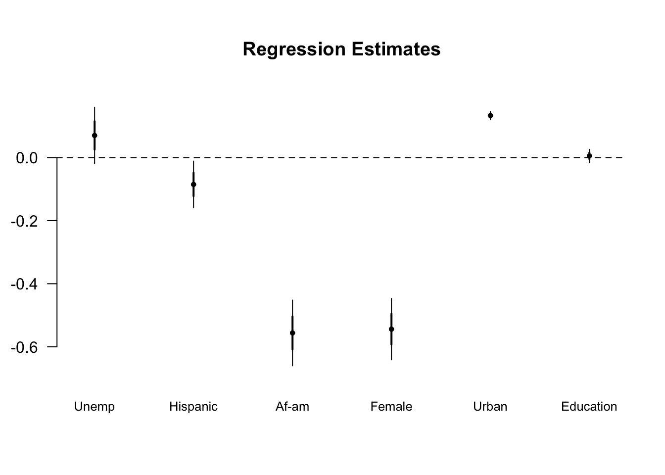

# after IV
coefplot(simple.ed.2s , vertical=FALSE, var.las=1, varnames=c("Education","Unemp","Hispanic","Af-am","Female","Urban","Education"))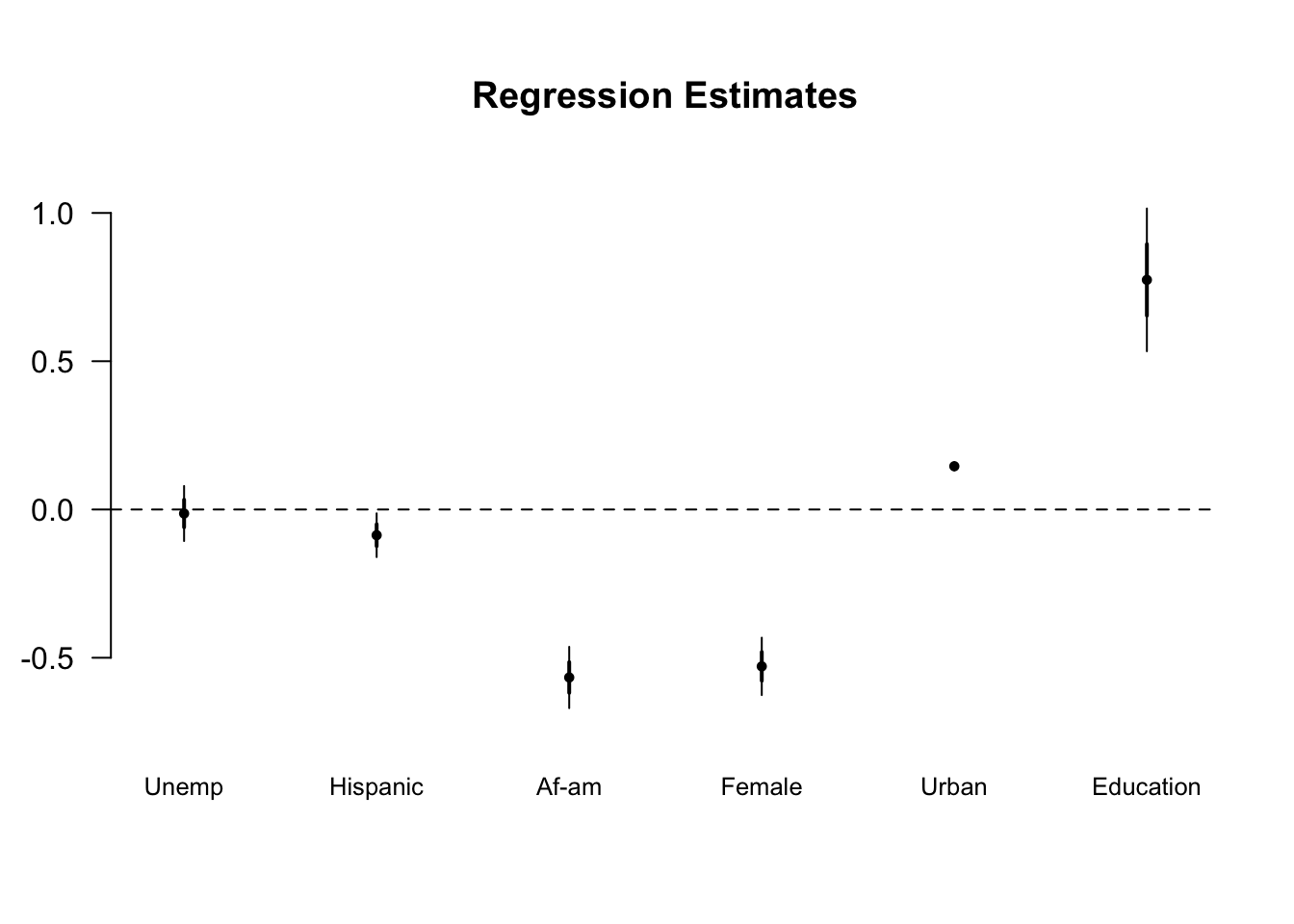

Inserting the predicted values of the first stage as a proxy for education in the second stage gives us a significant effect of education (instrumented by distance) on earnings.

The error on the computed parameter for education in our instrumental variable estimate is much larger than the simple OLS estimate. Part of this comes from OLS underestimating the variance but most of it comes from the added noise in generating a two-stage estimate. We’ll get back to that later.

simple.ed.endog <- lm(wage ~ urban + gender + ethnicity + unemp + education , data=cd.d)
simple.ed.2sls <- ivreg(wage ~ urban + gender + ethnicity + unemp + education | . - education + distance, data=cd.d)
stargazer(simple.ed.endog, simple.ed.2s, simple.ed.2sls,
                    title="Title: Regression Results",
                    align=TRUE,
                    type = "text",
                    style = "ajs", 
                    notes=""
                    )

## 
## Title: Regression Results
##                                                                  
## =================================================================
##                                               WAGE               
##                                         OLS          instrumental
##                                                        variable  
##                                     1         2           3      
## -----------------------------------------------------------------
## urbanyes                          .070      -.014        .046    
##                                  (.045)     (.046)      (.060)   
##                                                                  
## genderfemale                     -.085*     -.087*      -.071    
##                                  (.037)     (.037)      (.050)   
##                                                                  
## ethnicityafam                   -.556***   -.567***     -.227*   
##                                  (.052)     (.052)      (.099)   
##                                                                  
## ethnicityhispanic               -.544***   -.529***    -.351***  
##                                  (.049)     (.048)      (.077)   
##                                                                  
## unemp                            .133***   .146***     .139***   
##                                  (.007)     (.007)      (.009)   
##                                                                  
## education                         .005                 .647***   
##                                  (.010)                 (.136)   
##                                                                  
## ed.pred                                    .774***               
##                                             (.120)               
##                                                                  
## Constant                        8.641***    -2.054      -.359    
##                                  (.157)    (1.675)     (1.908)   
##                                                                  
## Observations                      4,739     4,739       4,739    
## R2                                .110       .117       -.612    
## Adjusted R2                       .109       .116       -.614    
## Residual Std. Error (df = 4732)   1.268     1.263       1.706    
## F Statistic (df = 6; 4732)      97.274*** 104.971***             
## -----------------------------------------------------------------
## Notes:                          *P < .05                         
##                                 **P < .01                        
##                                 ***P < .001                      
##

Twins and returns to schooling

Estimates of the returns to schooling for Twinsburg twins (Ashenfelter and Krueger, 1994); Ashenfelter and Rouse, 1998). (This replicates the analysis in Table 6.2 of Mastering ’Metrics.)

library("tidyverse")
library("sandwich")
library("lmtest")
library("AER")

Load twins data.

pubtwins <- read.csv("data/pubtwins.csv")
head(pubtwins)

##   X first educ educt    hrwage    lwage      age white female selfemp
## 1 1     1   16    16 11.935573 2.479523 33.25119     1      1       0
## 2 2    NA   16    16  9.208958 2.220177 33.25119     1      1       0
## 3 3    NA   12    16  9.283223 2.228209 43.57014     1      1       0
## 4 4     1   18    12 19.096916 2.949527 43.57014     1      1       0
## 5 5    NA   12    12 15.447336 2.728481 30.98391     1      0       0
## 6 6     1   12    12 17.432159 2.858290 30.98391     1      0       0
##   uncov married tenure nsibs daded momed educt_t educ_t  lwage_t      age2
## 1     0       0  3.000    NA    12    12      16     16 2.220177 1105.6416
## 2     0       0  1.667    NA    12    12      16     16 2.479523 1105.6416
## 3     1       1  7.000    NA    12    12      12     18 2.949527 1898.3575
## 4     1       1 10.000    NA    12    12      16     12 2.228209 1898.3575
## 5     1       1  8.500     6    12    12      12     12 2.858290  960.0026
## 6     0       1 10.000     6    12    12      12     12 2.728481  960.0026
##   twoplus aeduct     dlwage deduc deduct dceduc dceduct cseduc cseduct
## 1       0     16  0.2593465     0      0      0       0     16      16
## 2       0     16 -0.2593465     0      0      0       0     16      16
## 3       0     17 -0.7213180    -6     -4     -4      -6     14      15
## 4       0     12  0.7213180     6      4      6       4     15      14
## 5       1     12 -0.1298089     0      0      0       0     12      12
## 6       1     12  0.1298089     0      0      0       0     12      12
##   dcsumint dcsuminz duncov dmaried dtenure pedhs pedcl dcpedhs dcpedhst
## 1        0        0      0       0   1.333     1     0       0        0
## 2        0        0      0       0  -1.333     1     0       0        0
## 3      -56      -90      0       0  -3.000     1     0      -4       -6
## 4       90       56      0       0   3.000     1     0       6        4
## 5        0        0      1       0  -1.500     1     0       0        0
## 6        0        0     -1       0   1.500     1     0       0        0
##   dcpedcl dcpedclt
## 1       0        0
## 2       0        0
## 3       0        0
## 4       0        0
## 5       0        0
## 6       0        0

Run a regression of log wage on controls (Column 1 of Table 6.2).

mod1 <- lm(lwage ~ educ + poly(age,2) + female + white, data = pubtwins)
coeftest(mod1, vcov = sandwich)

## 
## t test of coefficients:
## 
##                Estimate Std. Error t value  Pr(>|t|)    
## (Intercept)    1.179124   0.163079  7.2304 1.311e-12 ***
## educ           0.109992   0.010431 10.5445 < 2.2e-16 ***
## poly(age, 2)1  4.964283   0.569685  8.7141 < 2.2e-16 ***
## poly(age, 2)2 -4.295745   0.591919 -7.2573 1.090e-12 ***
## female        -0.317994   0.039746 -8.0006 5.413e-15 ***
## white         -0.100095   0.067920 -1.4737     0.141    
## ---
## Signif. codes:  0 '***' 0.001 '**' 0.01 '*' 0.05 '.' 0.1 ' ' 1

Note: The age coefficients are different (but equivalent) to those reported in the Table due to the the use of poly(age,.), which calculates orthogonal polynomials.

Run regression of the difference in log wage between twins on the difference in education (Column 2 of Table 6.2).

mod2 <- lm(dlwage ~ deduc, data = filter(pubtwins, first == 1))
coeftest(mod2, vcov = sandwich)

## 
## t test of coefficients:
## 
##             Estimate Std. Error t value Pr(>|t|)   
## (Intercept) 0.029562   0.027520  1.0742 0.283498   
## deduc       0.061044   0.019768  3.0880 0.002182 **
## ---
## Signif. codes:  0 '***' 0.001 '**' 0.01 '*' 0.05 '.' 0.1 ' ' 1

Run a regression of log wage on controls, instrumenting education with twin’s education (Column 3 of Table 6.2).

mod3 <- ivreg(lwage ~ educ + poly(age,2) + female + white |
                . - educ + educt, data = pubtwins)
summary(mod3, vcov = sandwich, diagnostics = TRUE)

## 
## Call:
## ivreg(formula = lwage ~ educ + poly(age, 2) + female + white | 
##     . - educ + educt, data = pubtwins)
## 
## Residuals:
##      Min       1Q   Median       3Q      Max 
## -1.69585 -0.29218  0.00494  0.26262  2.47060 
## 
## Coefficients:
##               Estimate Std. Error t value Pr(>|t|)    
## (Intercept)    1.06356    0.21125   5.035 6.15e-07 ***
## educ           0.11792    0.01368   8.620  < 2e-16 ***
## poly(age, 2)1  5.03666    0.58054   8.676  < 2e-16 ***
## poly(age, 2)2 -4.28974    0.59284  -7.236 1.26e-12 ***
## female        -0.31490    0.04031  -7.812 2.16e-14 ***
## white         -0.09738    0.06820  -1.428    0.154    
## 
## Diagnostic tests:
##                  df1 df2 statistic p-value    
## Weak instruments   1 674   796.295  <2e-16 ***
## Wu-Hausman         1 673     0.916   0.339    
## Sargan             0  NA        NA      NA    
## ---
## Signif. codes:  0 '***' 0.001 '**' 0.01 '*' 0.05 '.' 0.1 ' ' 1
## 
## Residual standard error: 0.507 on 674 degrees of freedom
## Multiple R-Squared: 0.3381,  Adjusted R-squared: 0.3332 
## Wald test: 56.76 on 5 and 674 DF,  p-value: < 2.2e-16

Run a regression of the difference in wage, instrumenting the difference in years of education with twin’s education (Column 4 of Table 6.2).

mod4 <- ivreg(dlwage ~ deduc | deduct,
              data = filter(pubtwins, first == 1))
summary(mod4, vcov = sandwich, diagnostics = TRUE)

## 
## Call:
## ivreg(formula = dlwage ~ deduc | deduct, data = filter(pubtwins, 
##     first == 1))
## 
## Residuals:
##      Min       1Q   Median       3Q      Max 
## -2.04226 -0.31113 -0.02735  0.24705  2.08239 
## 
## Coefficients:
##             Estimate Std. Error t value Pr(>|t|)   
## (Intercept)  0.02735    0.02768   0.988  0.32369   
## deduc        0.10701    0.03394   3.153  0.00176 **
## 
## Diagnostic tests:
##                  df1 df2 statistic p-value    
## Weak instruments   1 338    85.150  <2e-16 ***
## Wu-Hausman         1 337     4.122  0.0431 *  
## Sargan             0  NA        NA      NA    
## ---
## Signif. codes:  0 '***' 0.001 '**' 0.01 '*' 0.05 '.' 0.1 ' ' 1
## 
## Residual standard error: 0.5119 on 338 degrees of freedom
## Multiple R-Squared: 0.01322, Adjusted R-squared: 0.0103 
## Wald test: 9.944 on 1 and 338 DF,  p-value: 0.001759

References

https://jrnold.github.io/masteringmetrics

Weak instruments

What if $Cov(z,u)\ne0$?

The IV estimator will also be inconsistent (as is OLS)

Compare the asymptotic bias in OLS to that in IV: \[OLS: plim \hat \beta = \beta + corr(x,u)\frac{\sigma_u}{\sigma_x}\] \[IV: plim \hat \beta = \beta + \frac{corr(z,u)}{corr(z,x)}\frac{\sigma_u}{\sigma_x}\] Even if $corr(z,u)$ is small, the inconsistency can be large if $corr(z,x)$ is also very small.

It is not necessarily better to use IV over OLS, even if $z$ and $u$ are not highly correlated.
- Instead, prefer IV only if $\frac{corr(z,u)}{corr(z,x)}<corr(x,u)$.

Think of it this way: An instrument that is not “fully” excludable can become a big problem if $cov(z,x)$ is small… we fear weak instruments to the extent we aren’t sure of the validity of the exclusion restriction.

Heterogeneous treatment effects

The implicit baseline model here is a model of common treatment effects. That is, there is an indicator variable for the treatment and everyone has the same value for the coefficient on this variable. If one is ambitious, the dummy variable might be interacted with various observable characteristics to estimate subgroup effects. (Similar issues arise with random coefficient models for continuous independent variables of interest.)

In the case of IV, the key issue that has excited the most attention is the potential for instruments that are uncorrelated with the error term (of the outcome equation) to nonetheless be correlated with the person-specific component of the impact.

The linear model

Consider the equation \[Y_i=\beta X_i+\delta_i D_i+\epsilon_i ,\] where the :$i$" subscript on the indicator variable is suggestive of heterogeneous treatment effects. Now, let \[\delta_i = {\bar \delta} + \delta_i^*,\] where we decompose the individual treatment effect into the mean treatment effect, ${\bar \delta}$, and the individual deviation from that mean, $\delta_i^*$. We can then re-write the model as \[Y_i=\beta X_i+{\bar \delta} D_i+\delta_i^* D_i +\epsilon_i,\] where $(\delta_i^* D_i +\epsilon_i)$ is the composite error term. For the untreated units, this error term consists only of the usual error term. For the treated units, however, it consists of both the usual error term and the idiosyncratic component of the treatment.

In the common-coefficient model, the condition for a valid instrument is \[E(\epsilon_i | X_i,D_i,Z_i)=0.\] In contrast, the corresponding condition for the heterogeneous-treatment effect world is given by \[E[(\delta_i^* D_i + \epsilon_i) | X_i,D_i,Z_i]=0.\] This is a different (and stronger) condition that will not be satisfied by many standard instruments.

To see why, consider a typical IV strategy in a treatment-effects context. Suppose that variation in the cost of treatment is to be used to generate exogenous variation in the probability of treatment. If the component of cost that generates the variation (e.g., distance from the training center) is uncorrelated with the outcome-equation residual, then this constitutes a valid instrument in the common-effect world. However, it is easy to show that such instruments are not likely to be valid in the heterogeneous-treatment-effects world, if agents know both their costs and their likely impacts from the program.

Suppose that participation is determined by \[D_i^*=\gamma_0 + \gamma_1 \delta_1 +\gamma_2 Z_i + v_i,\] where $D_i = 1$ iff $D_i^* > 0$ and $D_i=0$ otherwise, and where $Z_i$ is a variable that measures the cost of participation. In this case, units with high idiosyncratic impacts will participate even when their costs are high, but units with low idiosyncratic impacts will participate only when their costs are low. As a result—and this is the key point – conditional on $D$, the value of the instrument is correlated with the unit-specific component of the impact. Put differently, the standard model of participation—based on the model in Heckman and Robb (J of Econometrics 1985)—implies that cost-based instruments are likely invalid in a heterogeneous treatment effects world. (In terms of notation, in this case $E[(\delta_i-{\bar \delta})| X_i,D_i,Z_i] \ne 0$.)

This being the case, all is not lost. When the instrument is correlated with the unit-specific component of the impact but not with the error term in the original outcome equation, IV still estimates an interpretable and (sometimes) useful parameter under some additional assumptions.

Local average treatment effects

It is easiest to see what is going on with local average treatment effects (LATE) if we stick to the very simple case of a binary instrument, a binary treatment, and no covariates.

Consider four groups of observed subjects and the binary instrument, $Z$. The “Compliers” are the key group here. They are the units that respond to the instrument by taking the treatment when they otherwise would not have. (For example, if costs are the instrument, these units do not participate when costs are high but do participate when costs are low.)

The values of the treatment variable, $D$, for values of the instrument, $Z$

Subjects	$Z=0$	$Z=1$
Never takers (NT)	0	0
Defiers (DF)	1	0
Compliers (C)	0	1
Always takers (AT)	1	1

Now consider the formula for the Wald estimator once again: \[\Delta_{IV}=\frac{E(Y | Z=1)-E(Y | Z=0)}{Pr(D=1 | Z = 1) - Pr(D=1 | Z = 0)}.\] Using these four groups, we can rewrite the terms in the numerator as

and

The denominator terms become

$Pr(D=1| Z=1)= Pr(D=1|Z=1,AT)Pr(AT)+Pr(D=1|Z=1,C)Pr(C) = Pr(AT)+Pr(C)$

and

$Pr(D=1|Z=0) = Pr(D=1|Z=0,AT)Pr(AT) + Pr(D=1|Z=0,DF)Pr(DF) = Pr(AT)+Pr(DF)$

Some of these terms cancel out, leaving

\[\Delta_{IV}= \frac{[E(Y_1|C)Pr(C)-E(Y_0|C)Pr(C)]-[E(Y_0|DF)Pr(DF)-E(Y_1|DF)Pr(DF)]}{Pr(C)-Pr(DF)}.\]

This is a bit of a mess, but still provides some insight. The IV estimator in this case is a weighted average of the treatment effect on the compliers and the negative of the treatment effect on the defiers. (Note also that as $Pr(DF)\rightarrow 0$, $\Delta_{IV}\rightarrow E(Y_1|C)-E(Y_0|C)$.) This is contributed to by “Compliers” and “Always takers,” while $Pr(D=1 | Z = 0)$ is contributed to by “Defiers” and “Never takers.” Thus, to the extent the sample of those exposed to $Z=1$ consists of “Compliers,” $Pr(D=1 | Z = 1)$ approaches 1. Likewise, to the extent the sample of those exposed to $Z=0$ consists of “Defiers,” $Pr(D=1 | Z = 0)$ also approaches 1. All else equal, this drives ${\hat \Delta_{IV}}$ upward.

To get from here to the LATE, two assumptions are required.

Monotonicity: That is, we assume that the instrument can only increase or decrease the probabilities of participation. Thus, if increasing the instrument increases the probability of participation for some units, it does so for all. This assumption fits in very well for cost-based instruments, which theory suggests should have such a monotonic effect.
- In terms of the notation, monotonicity implies that $Pr(DF) = 0$… i.e., there are no defiers.
There are some compliers: The behavior of some individuals must be affected by the instrument (which is to say $Pr(C) > 0$).

Imposing these assumptions on the formula gives (the LATE):

\[\Delta_{IV}= \frac{E(Y_1|C)Pr(C)-E(Y_0|C)Pr(C)}{Pr(C)}=E(Y_1|C)-E(Y_0|C).\]

Thus, in a heterogeneous-treatment-effects world—where the instrument is correlated with the impact and where monotonicity holds—the IV estimator gives the Local Average Treatment Effect (LATE), defined as the mean impact of treatment on the compliers.

The LATE is a well-defined economic parameter. In some cases, as when the available policy option consists of moving the instrument, it may be the parameter of greatest interest. Thus, if we consider giving a $500 tax credit for university attendance, the policy parameter of interest is the impact of university on individuals who attend with the tax credit but do not attend without it.

The LATE provides no information about the impact of treatment on the “always takers,” which could be large or small. If the mean impact of treatment on the treated is the primary parameter of interest, this is a very important omission.

(Note how this works in the JTPA experiment with dropouts and substitutes – 60 percent treated in the treatment group and 40 percent treated in the control group. The impact estimate when you do the Wald/Bloom estimator is a LATE. It is the impact on the 20 percent who receive treatment because they were randomly assigned into the treatment group rather than the control group.)

Revisiting the distance example

Return now to our simple example of the two training centers, but change the parameters as follows:

Outcome in the absence of training: $100
Tuition for the training course: 5
Cost of travel from near town: 0
Cost of travel from far town: 10
Number of persons in each town: 100

Change the impacts so that they vary across persons. In particular, assume that:

Impact of training for one half of the population: $20
Impact of training for the other half of the population: 10

Assume also that the impact of training is independent of what town one lives in and that this impact from training is known by each individual. As before, $Z =1$ denotes residence in the near town and $Z = 0$ denotes residence in the far town.

Now we have the following:

\[Pr(D=1|Z=1) =1.0\] \[Pr(D=1|Z=0)=0.5\]

The latter follows from the fact that in the far town only those with an impact of 20 will take the training, because only for them does the impact exceed the combined travel and tuition costs. Similarly,

\[E(Y|Z =1)=Y_0 +E(\Delta|Z =1)Pr(D=1|Z =1)= 100 +[10(0.5)+20(0.5)]1=115,\]

and

\[E(Y |Z =0) =Y_0 +E(\Delta|Z =0) Pr(D=1|Z =0) = 100 + 20(0.5) =110.\]

Inserting the numbers from the example into the Wald formula gives:

\[{\hat \Delta_{IV}}=\frac{115 - 110}{1.0 - 0.5}=\frac{5}{0.5}=10,\]

This is the same answer as before, but now it is a local average treatment effect. The marginal group, the group that enters training when the instrument changes, consists of persons with impacts of 10. They participate in the near town but not in the far town.

Note that the LATE does not equal either the average treatment effect (ATE) or the treatment on the treated (TT). In particular,

\[\Delta^{ATE} =E(\Delta|Z=1)Pr(Z=1)+E(\Delta|Z=0)Pr(Z=0),\]

and

\[\Delta^{TT} =E(\Delta|Z=1,D=1)Pr(Z=1|D=1)+E(\Delta|Z=0,D=1)Pr(Z=0|D=1).\]

That is, these parameters are weighted averages of the mean impacts in each town, where the weights depend on the number of assumed participants in each town.

By assumption, $E(\Delta|Z=1)=10\times0.5+20\times0.5=15$.

By assumption, $E(\Delta|Z=0)=0\times0.5+20\times0.5=10$.

By assumption, $Pr(Z=1) = Pr(Z= 0) = 0.5$.

Also, $E(\Delta|Z=1,D=1)=10\times0.5+20\times0.5=15$, and $E(\Delta |Z=0,D=1)=20$ (due to differential participation).

Finally, $Pr(Z=1|D=1)=0.67$ while $Pr(Z=0|D=1) = 0.33$.

Thus,

\[\Delta^{ATE} =(15)(0.5)+(10)(0.5)=12.50,\]

and

\[\Delta^{TT} =(15)(0.67)+(20)(0.33) =16.65.\]

As expected, we have that $\Delta^{TT} > \Delta^{ATE}$.

Heterogeneous effects: Multiple instruments

In a world with heterogeneous treatment effects, the use of multiple instruments affects the nature of the parameter being estimated if the instruments are associated with the treatment effects.

Consider the case of two valid instruments, each of which is uncorrelated with the level but correlated with the impact. Each instrument, used separately, produces an estimate of a different LATE. Put differently, using each instrument estimates a different parameter.

Using both instruments together in 2SLS then produces a hybrid of the two LATEs. Again, a detailed treatment is beyond our scope here, but it is important to be aware that using multiple instruments changes from a simple and obviously useful way to improve the efficiency of the estimator to a complicated decision regarding the nature and definition of the parameter being estimated when the world switches from a homogeneous treatment effects world to a heterogeneous treatment effects world.

When different instruments estimate different LATEs, this also complicates the interpretation of Durbin-Wu-Hausman tests of over-identifying restrictions. Getting a different estimate when using two instruments rather than one of the two now no longer necessarily signals that the marginal

Where to get IVs

Theory combined with clever data collection: Theory can be used to come up with a variable that may affect participation but not outcomes other than through participation. Think about which variables might affect treatment choice but not have a direct effect on outcomes in the context of a formal or informal theory of the phenomenon being analyzed. Then find a data set, or collect some data, that embody these variables along with the outcomes and other exogenous co-variates. In many contexts such variables will represents aspects of the costs of being treated that are more or less exogenously assigned. (Most of these instruments yield local average treatment effects (LATEs) rather than ATE.)

Distance from a training center
Distance from college at birth, as in Card (1995)
Living in a town when/where a new college opens

Exogenous variation in policies or program implementation: A second source of instruments is exogenous variation in policy or program implementation. This can include variation over time or variation across space. The key is making the case that the variation really is exogenous. (These again will often yield LATEs rather than ATETs.)

Random assignment to judges of varying severity
Assignment to different caseworkers within a job training center

Nature: The natural world sometimes creates exogenous variation. Thus, learning about the natural world can have a payoff in economics.

Miscarriages and single motherhood, as in Hotz, Mullin, and Sanders (REStud 1997)
Temperature and fertility
Weather and fish
Sex of first two children for third birth
Twins as second birth for third child

Deliberate creation: A final source of instruments is deliberate creation. Running an experiment is one way of creating a really good instrument. When experiments are not feasible, Angrist and others have suggested randomized encouragement as a method for creating a good instrument. The trick in this case is finding an outreach technique that has a substantial effect on the probability of participation.

Literature

Consider Angrist (AER 1990), Angrist and Krueger (QJE 1991), Ashenfelter and Krueger (AER 1994), Angrist and Evans (AER 1998).

Micro-Econometrics