Chapter 11 Synthetic controls
Running synnthetic controls in R
library("Synth")
## Second example: The economic impact of terrorism in the
## Basque country using data from Abadie and Gardeazabal (2003)
## see JSS paper in the references details

data(basque)

# dataprep: prepare data for synth
dataprep.out <-
  dataprep(
  foo = basque
  ,predictors= c("school.illit",
                 "school.prim",
                 "school.med",
                 "school.high",
                 "school.post.high"
                 ,"invest"
                 )
   ,predictors.op = c("mean")
   ,dependent     = c("gdpcap")
   ,unit.variable = c("regionno")
   ,time.variable = c("year")
   ,special.predictors = list(
    list("gdpcap",1960:1969,c("mean")),
    list("sec.agriculture",seq(1961,1969,2),c("mean")),
    list("sec.energy",seq(1961,1969,2),c("mean")),
    list("sec.industry",seq(1961,1969,2),c("mean")),
    list("sec.construction",seq(1961,1969,2),c("mean")),
    list("sec.services.venta",seq(1961,1969,2),c("mean")),
    list("sec.services.nonventa",seq(1961,1969,2),c("mean")),
    list("popdens",1969,c("mean")))
    ,treatment.identifier  = 17
    ,controls.identifier   = c(2:16,18)
    ,time.predictors.prior = c(1964:1969)
    ,time.optimize.ssr     = c(1960:1969)
    ,unit.names.variable   = c("regionname")
    ,time.plot            = c(1955:1997)
    )

# 1. combine highest and second-highest schooling category
# and eliminate highest category
dataprep.out$X1["school.high",] <-
 dataprep.out$X1["school.high",] +
 dataprep.out$X1["school.post.high",]
dataprep.out$X1                 <-
 as.matrix(dataprep.out$X1[
  -which(rownames(dataprep.out$X1)=="school.post.high"),])
dataprep.out$X0["school.high",] <-
 dataprep.out$X0["school.high",] +
 dataprep.out$X0["school.post.high",]
dataprep.out$X0                 <-
dataprep.out$X0[
 -which(rownames(dataprep.out$X0)=="school.post.high"),]

# 2. make total and compute shares for the schooling catgeories
lowest  <- which(rownames(dataprep.out$X0)=="school.illit")
highest <- which(rownames(dataprep.out$X0)=="school.high")

dataprep.out$X1[lowest:highest,] <-
 (100 * dataprep.out$X1[lowest:highest,]) /
 sum(dataprep.out$X1[lowest:highest,])
dataprep.out$X0[lowest:highest,] <-
 100 * scale(dataprep.out$X0[lowest:highest,],
             center=FALSE,
             scale=colSums(dataprep.out$X0[lowest:highest,])
                                                 )

# run synth
synth.out <- synth(data.prep.obj = dataprep.out)
##
## X1, X0, Z1, Z0 all come directly from dataprep object.
##
##
## ****************
## searching for synthetic control unit
##
##
## ****************
## ****************
## ****************
##
## MSPE (LOSS V): 0.008864629
##
## solution.v:
## 0.01556808 0.001791073 0.04417159 0.03409436 8.45034e-05 0.2009837 0.09484593 0.007689228 0.1339499 0.008723843 0.009680725 0.1081258 0.3402913
##
## solution.w:
## 4.92e-08 5.17e-08 1.352e-07 2.85e-08 5.32e-08 5.177e-07 5.24e-08 7.29e-08 0.8507986 2.274e-07 4.03e-08 9.51e-08 0.1491998 5.61e-08 9.02e-08 1.061e-07# Get result tables
synth.tables <- synth.tab(
dataprep.res = dataprep.out,
synth.res = synth.out
)
# results tables:
print(synth.tables)## $tab.pred
## Treated Synthetic Sample Mean
## school.illit 3.321 7.645 10.983
## school.prim 85.893 82.285 80.911
## school.med 7.522 6.965 5.427
## school.high 3.264 3.105 2.679
## invest 24.647 21.583 21.424
## special.gdpcap.1960.1969 5.285 5.271 3.581
## special.sec.agriculture.1961.1969 6.844 6.179 21.353
## special.sec.energy.1961.1969 4.106 2.760 5.310
## special.sec.industry.1961.1969 45.082 37.636 22.425
## special.sec.construction.1961.1969 6.150 6.952 7.276
## special.sec.services.venta.1961.1969 33.754 41.104 36.528
## special.sec.services.nonventa.1961.1969 4.072 5.371 7.111
## special.popdens.1969 246.890 196.288 99.414
##
## $tab.v
## v.weights
## school.illit 0.016
## school.prim 0.002
## school.med 0.044
## school.high 0.034
## invest 0
## special.gdpcap.1960.1969 0.201
## special.sec.agriculture.1961.1969 0.095
## special.sec.energy.1961.1969 0.008
## special.sec.industry.1961.1969 0.134
## special.sec.construction.1961.1969 0.009
## special.sec.services.venta.1961.1969 0.01
## special.sec.services.nonventa.1961.1969 0.108
## special.popdens.1969 0.34
##
## $tab.w
## w.weights unit.names unit.numbers
## 2 0.000 Andalucia 2
## 3 0.000 Aragon 3
## 4 0.000 Principado De Asturias 4
## 5 0.000 Baleares (Islas) 5
## 6 0.000 Canarias 6
## 7 0.000 Cantabria 7
## 8 0.000 Castilla Y Leon 8
## 9 0.000 Castilla-La Mancha 9
## 10 0.851 Cataluna 10
## 11 0.000 Comunidad Valenciana 11
## 12 0.000 Extremadura 12
## 13 0.000 Galicia 13
## 14 0.149 Madrid (Comunidad De) 14
## 15 0.000 Murcia (Region de) 15
## 16 0.000 Navarra (Comunidad Foral De) 16
## 18 0.000 Rioja (La) 18
##
## $tab.loss
## Loss W Loss V
## [1,] 0.2466976 0.008864629# plot results:
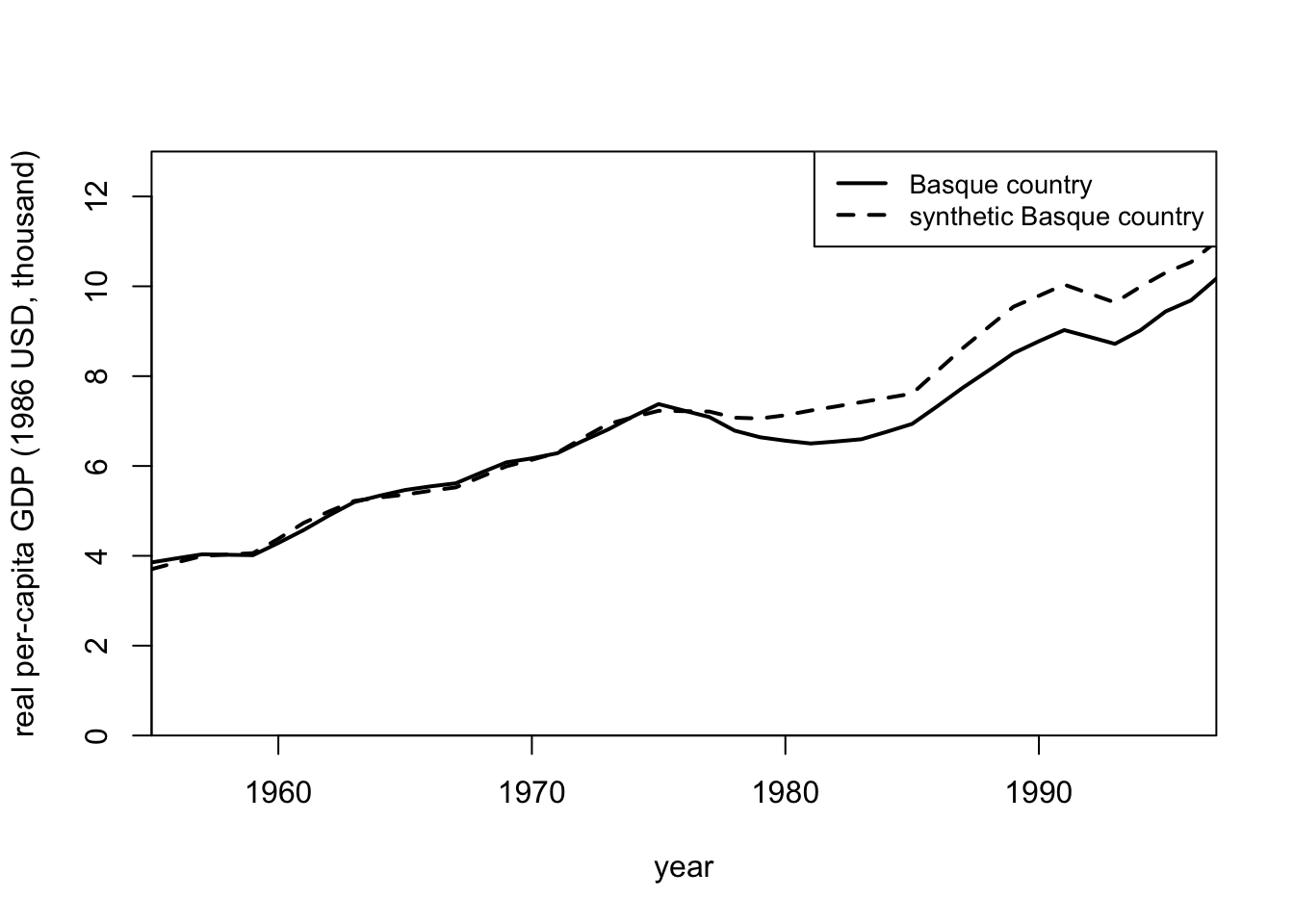
# path
path.plot(synth.res = synth.out,
dataprep.res = dataprep.out,
Ylab = c("real per-capita GDP (1986 USD, thousand)"),
Xlab = c("year"),
Ylim = c(0,13),
Legend = c("Basque country","synthetic Basque country"),
) 
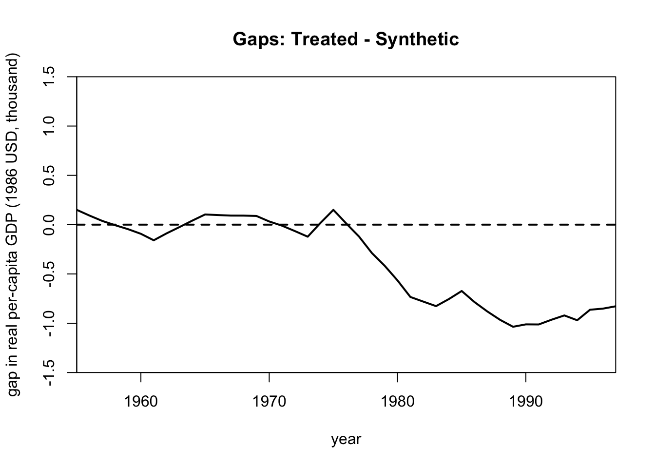
## gaps
gaps.plot(synth.res = synth.out,
          dataprep.res = dataprep.out,
          Ylab = c("gap in real per-capita GDP (1986 USD, thousand)"),
          Xlab = c("year"),
          Ylim = c(-1.5,1.5),
          )