Chapter 5 Notes on OLS

Why the constant term?

The SLR model is a population model. When it comes to estimating \(\beta_1\) (and \(\beta_0\)) using a random sample of data, we must restrict how \(u\) and \(x\) are related to each other.

What we must do is restrict the way \(u\) and \(x\) relate to each other in the population.

Taking the simple linear regression (SLR) model as given, \[y = \beta_0 + \beta_1x + u\], we will make a simplifying assumption: \[E(u)=0\] That is, the average value of \(u\) is zero in the population.

Note then, that it is the presence of \(\beta_0\) in \(y = \beta_0 + \beta_1x + u\) that allows us to assume \(E(u) = 0\) without loss of generality.

If the average of \(u\) was different from zero, say \(\alpha_0\), we would just adjust the intercept, which leaves the slope unchanged: \[y = (\beta_0 + \alpha_0) + \beta_1x + (u-\alpha_0)\]
The new error is: \(u - \alpha_0\)
The new intercept is: \(\beta_0 + \alpha_0\)

Importantly, note that what we care about knowing (i.e., \(\beta_1\)) is invariant to \(\alpha_0\)

What matters more, though…

… what matters for the inference we can make is that the mean of the error term does not change across different values of \(x\) in the population: \[E(u | x)=E(u) \hspace{2mm}\forall \hspace{2mm} x\]

If \(E(u | x)=E(u)\) for all \(x\), then \(u\) is mean independent of \(x\).

For example

Suppose you are interested in some \[Income=\beta_0 + \beta_1(schooling) + u\]

In \(u\) would be “ability,” then, yes? Mean independence would require that, \[E(ability | x = 8) = E(ability | x = 12) = E(ability | x = 16)\]

That is, the average ability should be the same across levels of education.

But, surely people choose education levels partly based on ability, yes? (We’ll return to this.)

Combining \(E(u | x) = E(u)\) (the substantive assumption) with \(E(u) = 0\) (a normalization) gives \[E(u | x)=0 \hspace{2mm}\forall \hspace{2mm} x.\]

We refer to this as the zero conditional mean assumption.
Because the conditional expected value is a linear operator, \(E(u | x) = 0\) implies \[E(y | x)= \beta_0 +\beta_1 x,\] which implies that the conditional expectation function (or population regression function) is a linear function of \(x\).

How can we estimate the population parameters, \(\beta_0\) and \(\beta_1\)?

Let \(\{f(x_i ; y_i ) : i = 1, 2, ... ; n\}\) be a random sample of size \(n\) (the number of observations) from the population.
Plug any \(i^{th}\) observation into the population equation: \[y_i = \beta_0 + \beta_1x_i + u_i,\] where the \(i\) subscript indicates a particular observation.
Note: We observe \(y_i\) and \(x_i\), but we do not observe \(u_i\) (though we know it is there).

To obtain estimating equations for \(\beta_0\) and \(\beta_1\), use the two population restrictions: \[E(u) = 0\] \[Cov(x,u) = 0\]

We talked about the first condition. The second condition, that the covariance is zero, means that \(x\) and \(u\) are uncorrelated. Both conditions are implied by \(E(u | x) = 0\).

Fitted values: For any candidates \({\hat \beta}_0\) and \({\hat \beta}_1\), define the fitted value for each \(i\) as \[{\hat y}_i = {\hat \beta}_0 + {\hat \beta}_1x_i\] There are \(n\) of these fitted values… the values we predict for \(y_i\) given \(x_i\). \end{frame}

Residuals: The “mistakes” we make in predicting \(y_i\) is the residual, \[{\hat u}_i = y_i - {\hat y}_i = y_i - ({\hat \beta}_0 + {\hat \beta}_1x_i)\]

We want to track both overshooting and undershooting \(y\). So… we measure the size of the “mistakes” across all \(i\) in the sample by first squaring them, and then summing across \(i\):\[\sum_{i=1}^{n}{\hat u}_i^2 = \sum_{i=1}^{n}(y_i-{\hat \beta}_0 - {\hat \beta}_1x_i)^2\]

The OLS estimates are those \({\hat \beta}_0\) and \({\hat \beta}_1\) that minimize the sum of squared residuals (SSR).

Note… \({\hat \beta}_1\) is an estimate of the parameter \(\beta_1\), obtained for a specific sample.

Different samples will generate different estimates (of true \(\beta_1\)).

Unbiasedness: If we have an unbiased estimator, we could take as many random samples from a population as we wanted to, and the average (mean) of all the estimates from each of those samples would be equal to the true \(\beta\).

Zero Conditional Mean Assumption: In the population, the error term has zero mean given any value of the explanatory variable: \[E(u | x) = E(u) = 0\]

This is the key assumption implying that OLS is unbiased, with the “zero” not being important once we assume \(E(u | x)\) does not change with \(x\).

The problem with OLS?

The problem: We can compute OLS estimates whether or not the zero conditional mean assumption (i.e., \(E(u | x) = E(u) = 0\)) holds.

The bigger problem: We think the zero conditional mean assumption is a little hard to swallow.

Consider Anscombe’s Quartet, for example… four distinct data-generating processes, each yielding the same coefficient estimates in OLS (in this case, \(y=3+0.5x\)). In no way has the causal effect of \(x\) been identified in all four scenarios.

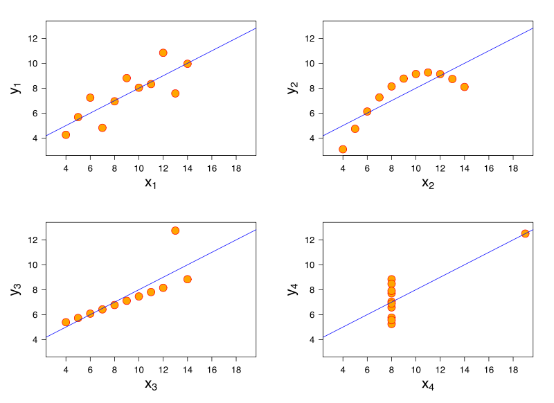Assumed in each: \(n=11, \mu_x=9, \mu_y=7.5, \sigma_x=11, \sigma_y=[4.122,4.127], \sigma_{xy}=0.816\)

Omitted-variable bias

Consider another example: \[ \mathbb{1}(working_i) = \beta_0 + \beta_1 numkids_i + u_i\]

If family size is random, then \(Cov(numkids_i, u_i)=0\), in which case \({\hat \beta}_1\) is the causal effect of \(numkids\) on \(working\).

Q: How do we interpret \({\hat \beta}_1\) if \(numkids\) is non-random? That is, what if \(Cov(numkids_i, u_i)\ne 0\)?

A: \({\hat \beta}_1\) is biased, where the sign if the bias is determined by \(Cov(x_i, u_i)\) and \(Cov(u_i, y_i)\).

The rule:

If \(Cov(u_i, y_i)\) & \(Cov(x_i, u_i)\) are similar in sign, the bias is positive.

If \(Cov(u_i, y_i)\) & \(Cov(x_i, u_i)\) are opposite in sign, the bias is negative.

An example

Q: What if 1) those with more kids also tend to be married (\(Cov(numkids_i, married_i)>0\)) and, 2) married people tend to be more likely to work (\(Cov(married_i, working_i)>0\))?

A: \({\hat \beta}_1\) is biased upward. (The effect of \(married\) is loading onto \(numkids\).)

Q: What if 1) black families tend to have more kids (\(Cov(numkids_i, black_i)>0\)) and 2) black employment tends to be lower (\(Cov(black_i, working_i)<0\))?

A: \({\hat \beta}_1\) is biased downward. (The effect of \(black\) is loading onto \(numkids\).)

So, if family size varies non-randomly… can we get to a place where we “believe” our \({\hat \beta}_1\)? That is… be comfortable assuming that family size is conditionally random? What would you want to condition on?

Anything that correlates with \(numkids\) and with \(working\).

\[\mathbb{1}(working_i) = \beta_0 + \beta_1 numkids_i + \gamma_1 married_i + \gamma_2 black_i + u_i\]

Here, if we want to estimate the average causal effect of family size on labor supply, the identifying assumption is

\(Cov(numkids_i, u_i)= 0\), or,
\(Cov(numkids_i, u_i | \{married_i, black_i\}) = 0\)

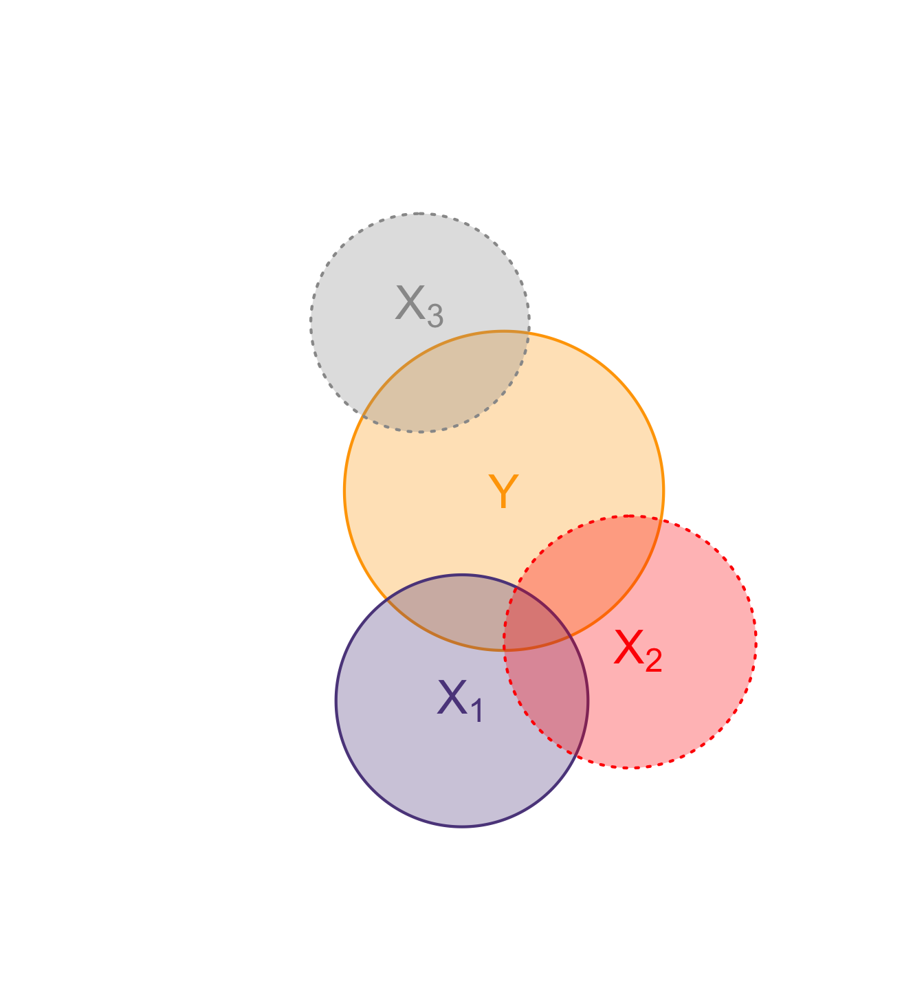
OVB in one picture

An abstraction for sure, but sometimes helpful. Consider these shapes representative of variation, and overlap therefore co-variation. The source of OVB in attributing the overlap of \(Y\) and \(X_1\) entirely to \(X_1\), as though causal, is the three-way overlap of \(Y\), \(X_1\), and \(X_2\), having run the model \(Y=\beta_0 + \beta_1 X_1 + u\).

In these figures (Venn diagrams)

Each circle illustrates a variable.
Overlap gives the share of correlatation between two variables.
Dotted borders denote omitted variables.