Chapter 8 Simulation

library(tidyverse)
library(broom)

When your intuition is exhausted, or your confidence is lacking… you need a tool. When your intuition is on point, but you also need a confidence boost… you need a tool. When you are writing estimators and you wish to demonstrate its properties… you need a tool.

Difference-in-differences model: The industry standard for causal identification (not gold standard… industry standard)

Difference-in-differences (DD) designs achieve causal identification, as all estimators do, by assumption. Here, that assumption is that the outcome variables of treated and control units trend similarly throughout the period of analysis.

In the standard setup, on could envision the following: \[y_{it} = y_{it} = X_i + T_t + \beta X_iT_t + \epsilon_i + \epsilon_t + \epsilon_{it},\]

were there is no allowance for uncommon trends. Suppose, however, that the true DGP was \[y_{it} = y_{it} = X_i + T_t + \beta X_iT_t + \delta tX_i + \epsilon_i + \epsilon_t + \epsilon_{it}.\]

Below, we will use this formulation and question the role of \(\delta\) as we will build our first simulated environments. We will do this first in R, and then in Stata.

Simulating DD in R

An R setup:

library(MonteCarlo)
library(latex2exp)
library(ggplot2)
library(plyr)
library(dplyr)
library(jtools)
library(ggstance)
library(ggthemes)
  theme_gw = theme_fivethirtyeight()+theme(plot.title = element_text(size=13, face="bold",margin = margin(10,0,10,0)))
library(AER)

The Function

dd_model <- function(beta, difftrend, n, var_i, var_t, var_it){
  # i-specific characteristics
  ind = 
    data.frame(
      i = 1:n,
      ei = rnorm(length(1:n), mean=0, sd=var_i),
      X = rep(0:1, each=n/2)
    )
  # make panel
  panel = ddply(ind, ~i, transform, t = 1:20) %>% 
    mutate(T = ifelse(t>10,1,0)) %>% 
    mutate(XT = X*T) 
  # error terms
  panel$eit = rnorm(dim(panel)[1], mean=0, sd=var_it)
  timeShock = 
    data.frame(
      t = 1:20,
      et = rnorm(length(1:20),mean=0, sd=var_t)
    )
  panel <- merge(panel,timeShock,by="t")
  panel = panel %>% mutate(y = X + T + beta * XT + 0 * t + difftrend * t * X + ei + et + eit)
  #panel <- panel[order(panel$i,panel$t),] 
  
  # run model
  model <- lm(y ~ X + T + XT, data=panel)
  betahat <- model$coefficients[4]
  betahat <- unname(betahat)
  return(list("betahat"=betahat))
}

The grids that cover parameter space

# define fixed parameter grids:
  n_grid<-c(100)
  var_i_grid<-c(1)
  var_t_grid<-c(1)
  var_it_grid<-c(1)
  beta_grid<-c(2)
# this is the parameter I am interested in varying, so I 
# specify the values over which MonteCarlo() run:
  difftrend_grid<-c(-.15,-.1,-.05,0,.05,.1,.15)

The simulation itself

The above was set up to test the implications of uncommon trends in a DD environment. Below, we now simply execute the intended simulation exercise.

  param_list=list("n"=n_grid, "var_i"=var_i_grid, "var_t"=var_t_grid, "var_it"=var_it_grid, "beta"=beta_grid, "difftrend"=difftrend_grid)
  mc_result <- MonteCarlo(func = dd_model, nrep = 500, param_list = param_list)

The presentation of results

Upon completion, we must extract results to prep for ggplot (or other) production of figures.

  summary(mc_result)
  df.mc<-MakeFrame(mc_result)
  head(df.mc)
  df.mc$difftrend <- as.factor(df.mc$difftrend)

---

1. Histrograms of parameter estimates, across the differential in \(T=1\) and \(T=0\) trends.

  ggplot(df.mc, aes(x=betahat, color=difftrend)) + 
  geom_histogram(binwidth=.03, alpha = 0.4, aes(y=..count../sum(..count..)), position = 'identity') +
  labs(color = TeX("$\\delta =$")) + 
  labs(title = TeX("Diff-in-Diff, $\\hat{\\beta}$ with and without common trends"),
      subtitle = TeX("$y_{it} = X_i + T_t + \\beta X_iT_t + \\delta tX_i + \\epsilon_i + \\epsilon_t + \\epsilon_{it}$"),
       caption = paste("Source: ",mc_result$meta$nrep," simulated samples of n=",n_grid,", with true treatment of ",mc_result$param_list$beta,sep="")) +
  theme_gw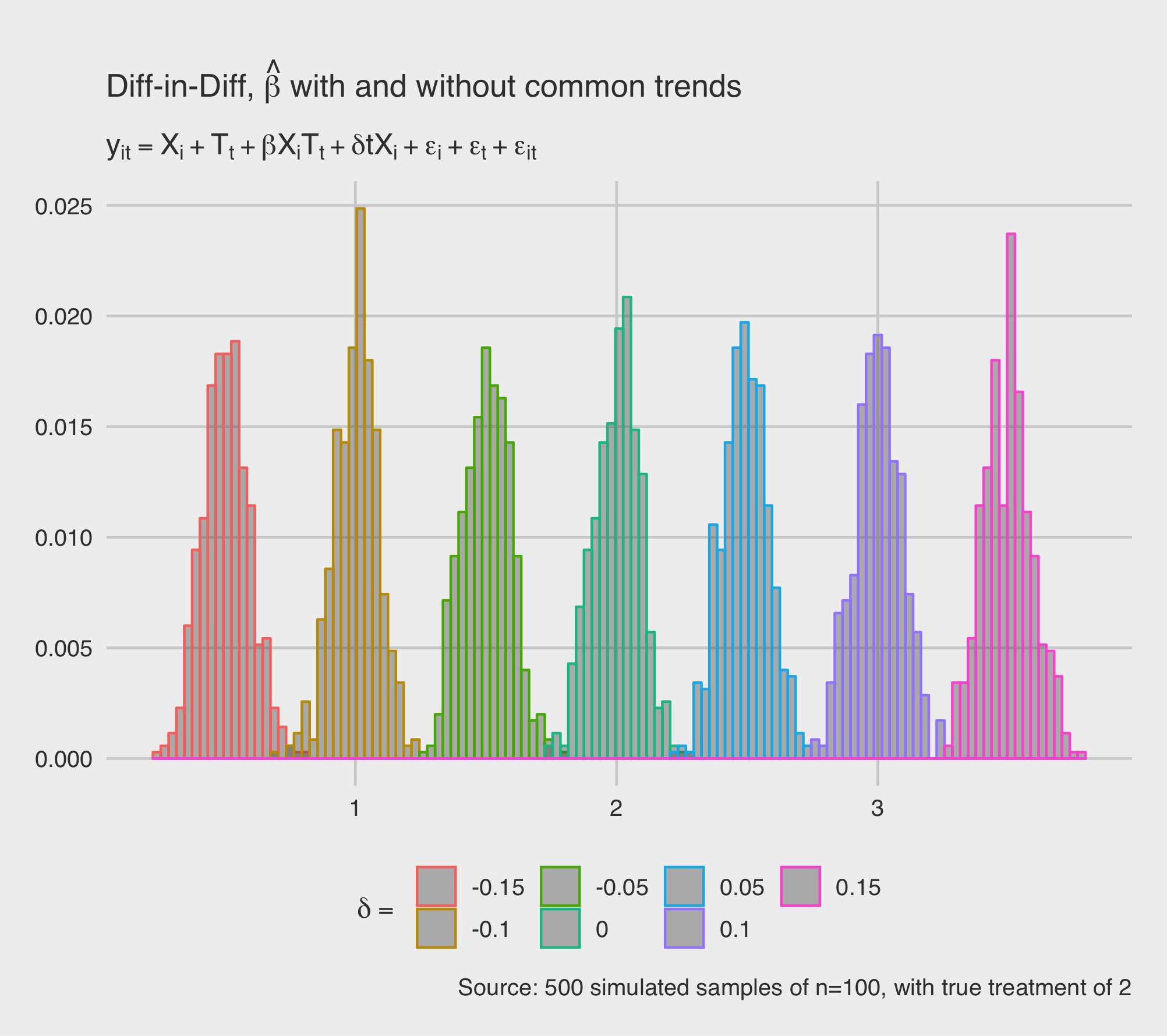

---

2. Box plots, parameter estimates, across the differential in \(T=1\) and \(T=0\) trends.

  ggplot(df.mc, aes(y=betahat, x=difftrend, color=difftrend)) + geom_boxplot() +
  geom_hline(aes(yintercept=mc_result$param_list$beta), color="black", linetype="solid", size=.5) +
  labs(color = TeX("$\\delta =$")) + scale_fill_manual(values=cbPalette) +
  labs(title = TeX("Diff-in-Diff, $\\hat{\\beta}$ with and without common trends"),
      subtitle = TeX("$y_{it} = X_i + T_t + \\beta X_iT_t + \\delta tX_i + \\epsilon_i + \\epsilon_t + \\epsilon_{it}$"),
       caption = paste("Source: ",mc_result$meta$nrep," simulated samples of n=",n_grid,", with true treatment of ",mc_result$param_list$beta,sep="")) +
  theme_gw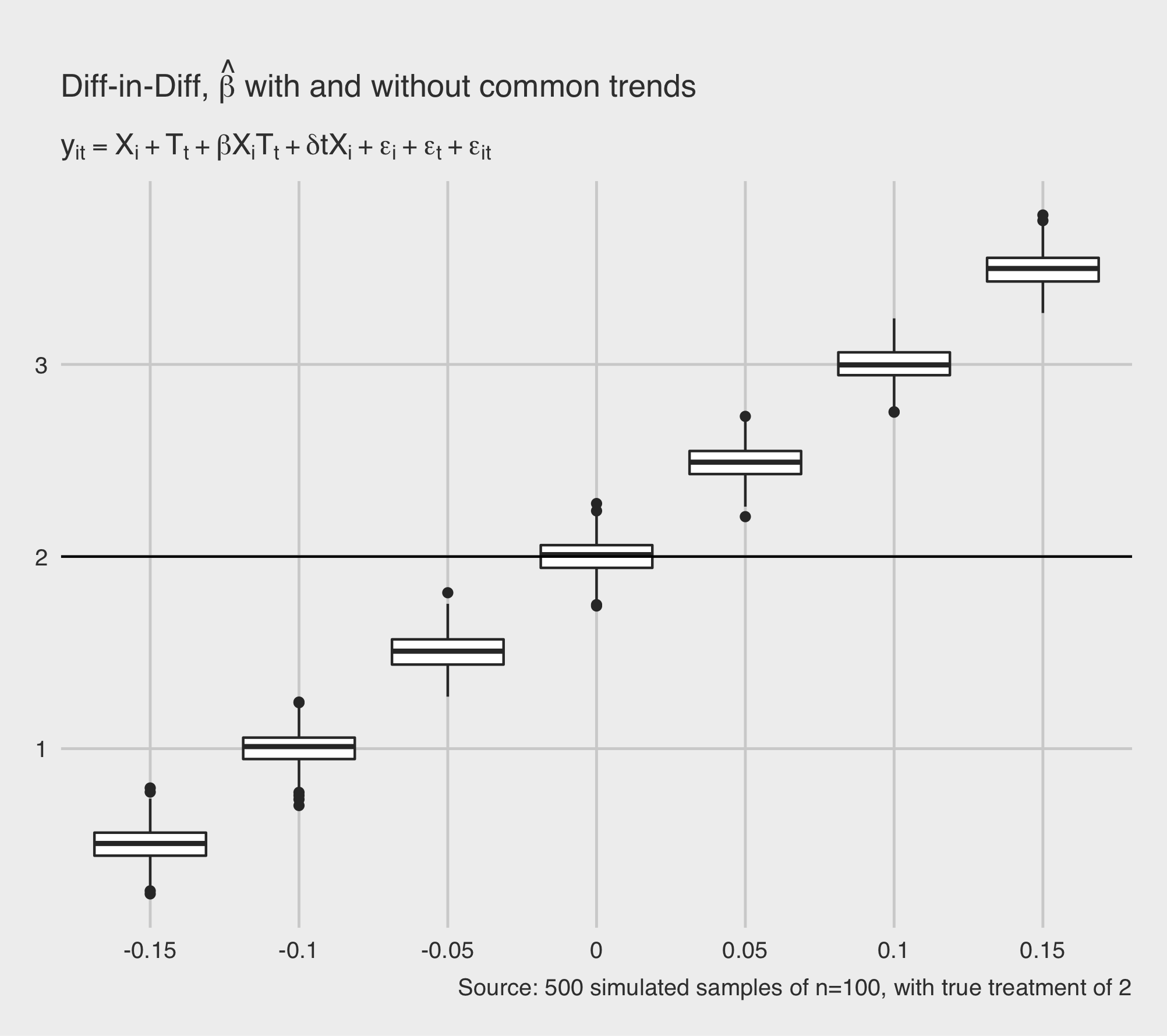

---

Simulating DD in Stata

Seting up the panel

glo people 100
glo years 10
set obs 2
ge X = _n-1
    label var X "Treatment group"
expand $years
qui bysort X: ge yr = _n
expand $people/2
qui bysort X yr: ge id = _n if X == 0   
qui bysort X yr: replace id = ($people/2)+_n if X == 1
ge T = 0
  replace T = 1 if yr > $years/2
    label var T "Treatment periods"
gen XT = X * T
gen y = .
order id yr X T XT
sort id yr
* in order to introduce differential trends
ge Xyr = X*yr
save EC607_Waddell_Metrics_structure.dta, replace

The program

glo reps = 100
glo truebeta = 1.5

capture program drop DD
program define DD, rclass
version 10.1
    syntax [, treatment(real 1.5) difftrend(real 0.0) ]
    drop _all
    use EC607_Waddell_Metric_structure.dta, clear
    gen e = rnormal(0,4)
    replace y = 1 + 2*X + 1.75*T + `treatment'*XT + e + `difftrend'*X*yr
    reg y X T XT
        return scalar bXT =_b[XT]
        return scalar seXT =_se[XT]
        return scalar t = (_b[XT]-`treatment')/_se[XT]
        return scalar r = abs(return(t))>invttail(_N-2,.025)
        return scalar p = 2*ttail(_N-2,abs(return(t)))
    return scalar treatment = `treatment' 
    return scalar difftrend = `difftrend' 
end

The simulation

The above was set up to test the implications of uncommon trends in a DD environment. Below, we now simply execute the intended simulation exercise.

glo tmin = -1
glo tmax = 1
glo j = 0
qui forv i = $tmin(.2)$tmax {
    glo j = $j + 1
    loc dt = `i' 
    simulate treatment=r(treatment) difftrend=r(difftrend) bXT=r(bXT) tXT=r(t) seXT=r(seXT) Preject=r(r), nolegend nodots saving(EC607_Waddell_Metrics_$j,replace) reps($reps): DD, treatment($truebeta) difftrend(`dt')
}

The presentation of results

Upon completion, we must extract results to prep for the production of figures.

use EC607_Waddell_Metrics_1, clear
erase EC607_Waddell_Metrics_1.dta
forv i=2/$j { 
    append using EC607_Waddell_Metrics_`i'
    erase EC607_Waddell_Metrics_`i'.dta
}

table difftrend, c(mean bXT mean Preject) f(%9.4f)

scatter bXT difftrend, msymbol(o) msize(vtiny) yline($truebeta) ti("Y = 1 + 2X + 1.25T + 1.5XT + e + Dtrend*Xt") yti(beta (true beta = 1.5)) xti("Dtrend")
    graph export EC607_Waddell_Metrics.png, replace

Can we simulate a dip?

Consider a small panel of \(n=10\), half of them treated commencing with period 11, with the DGP of:

\[y_{it} = \beta_0 + \beta_1X_i + \beta_2T_t + \beta_3 X_iT_t + \epsilon_{it}.\]

Can we simulate an Ashenfelter Dip?

set.seed(1972)
n=10; var_i=0; var_t=0; var_it=.2; beta0=5; beta1=-1; beta2=0; beta3=2;
  # i-specific characteristics
  ind = 
    data.frame(
      i = as.factor(1:n),
      ei = rnorm(length(1:n), mean=0, sd=var_i),
      X = rep(0:1, each=n/2)
    )
  # make panel
  panel = ddply(ind, ~i, transform, t = 1:20) %>% 
    mutate(T = ifelse(t>10,1,0)) %>% 
    mutate(XT = X*T) 
  # error terms
  panel$eit = rnorm(dim(panel)[1], mean=0, sd=var_it)
  timeShock = 
    data.frame(
      t = 1:20,
      et = rnorm(length(1:20),mean=0, sd=var_t)
    )
  panel <- merge(panel,timeShock,by="t")
  panel = panel %>% mutate(y = beta0 + beta1 * X + beta2 * T + beta3 * XT + eit)

  ggplot(data=panel, aes(x=t, y=y, group=i)) +
  geom_line(aes(color=i)) +
  geom_point(aes(color=i)) + theme_minimal()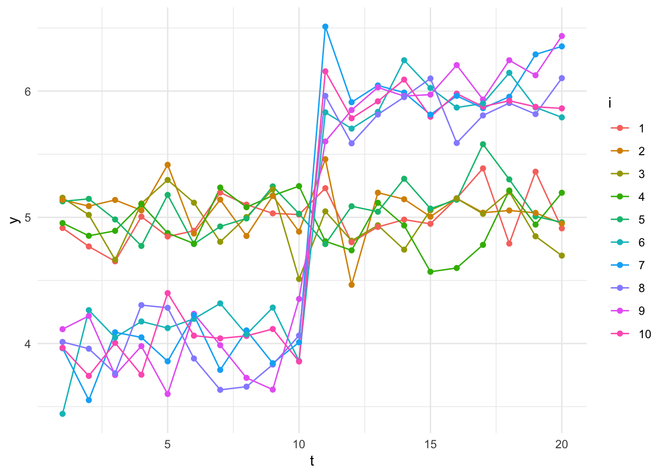

That last line before ggplot… where we created the outcome variable. Can we add a contaminated version of it?

dip9=.1; dip10=.2
panel = panel %>% mutate(ydip = ifelse(X==1 & t==9, y*(1-dip9), 
                                       ifelse(X==1 & t==10, y*(1-dip10), y)))

ggplot(data=panel, aes(x=t, y=ydip, group=i)) +
  geom_line(aes(color=X)) +
  geom_point(aes(color=X)) + 
  theme_minimal() + theme(legend.position="none")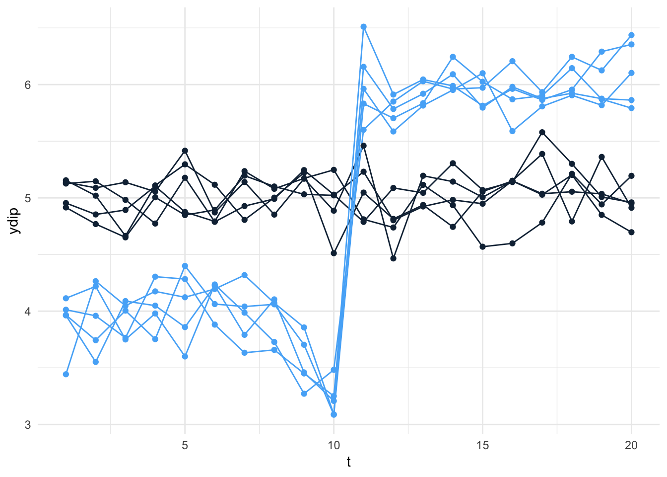

It would be nice to see the aggregate, so… here’s a function to set up the plotting of summary stats.

#+++++++++++++++++++++++++
# Function to calculate the mean and the standard deviation for each group
#+++++++++++++++++++++++++
# data : a data frame
# varname : the name of a column containing the variable to be summariezed
# groupnames : vector of column names to be used as grouping variables
data_summary <- function(data, varname, groupnames){
  require(plyr)
  summary_func <- function(x, col){
    c(mean = mean(x[[col]], na.rm=TRUE),
      sd = sd(x[[col]], na.rm=TRUE))
  }
  data_sum<-ddply(data, groupnames, .fun=summary_func,
                  varname)
  data_sum <- rename(data_sum, c("mean" = varname))
 return(data_sum)
}

We can then call this function as follows:

panel.sum <- data_summary(panel, varname="ydip", 
                    groupnames=c("X","t"))
head(panel.sum)

We can then plot the results.

ggplot(panel.sum, aes(x=t, y=ydip, group=X, color=X)) + 
    geom_errorbar(aes(ymin=ydip-sd, ymax=ydip+sd), width=.1, 
    position=position_dodge(0.05)) +
    geom_line() + geom_point() + 
    theme_minimal() + theme(legend.position="none")

OLS estimation of DD with (ash1) and without (ash0) Ashenfelter’s Dip.

ash1 <- lm(ydip ~ X + T + XT, panel)
summ(ash1, robust="HC1", confint=TRUE, digits=2)

Observations	200
Dependent variable	ydip
Type	OLS linear regression

F(3,196)	618.39
R²	0.90
Adj. R²	0.90

	Est.	2.5%	97.5%	t val.	p
(Intercept)	5.01	4.96	5.06	193.13	0.00	***
X	-1.14	-1.25	-1.04	-21.09	0.00	***
T	0.00	-0.08	0.09	0.10	0.92
XT	2.09	1.96	2.23	30.33	0.00	***
Standard errors: Robust, type = HC1

ash0 <- lm(y ~ X + T + XT, panel)
summ(ash0, robust="HC1", confint=TRUE, digits=2)

Observations	200
Dependent variable	y
Type	OLS linear regression

F(3,196)	738.02
R²	0.92
Adj. R²	0.92

	Est.	2.5%	97.5%	t val.	p
(Intercept)	5.01	4.96	5.06	193.13	0.00	***
X	-1.02	-1.11	-0.94	-24.73	0.00	***
T	0.00	-0.08	0.09	0.10	0.92
XT	1.97	1.86	2.09	33.19	0.00	***
Standard errors: Robust, type = HC1

What about the sensitivity of the point estimate to the exclusion of those observations around treatment (ashhole)?

ashhole <- lm( ydip ~ X + T + XT, panel, t<=8 | t >=11 )
summ(ashhole, robust="HC1", confint=TRUE, digits=2)

Observations	180
Dependent variable	ydip
Type	OLS linear regression

F(3,176)	661.05
R²	0.92
Adj. R²	0.92

	Est.	2.5%	97.5%	t val.	p
(Intercept)	5.00	4.94	5.05	182.74	0.00	***
X	-1.01	-1.10	-0.92	-22.14	0.00	***
T	0.02	-0.07	0.10	0.36	0.72
XT	1.96	1.84	2.09	31.35	0.00	***
Standard errors: Robust, type = HC1

Comparing models, note the “need” for OLS to still fit the mean (so \({\hat \beta}_{X}\) is offsets \({\hat \beta}_{XT}\))

plot_summs(ash0, ash1, scale = TRUE, plot.distributions = TRUE)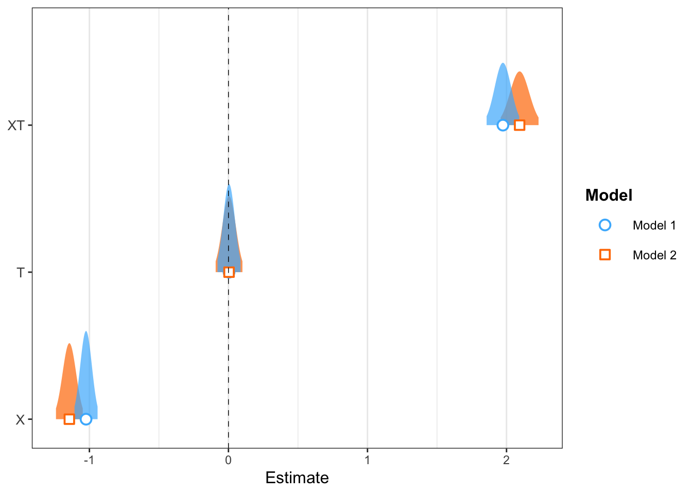

Note: Stargazer offers some nice options for tables.

stargazer(ash1, ashhole, type="text",
dep.var.labels=c("Dip","Dip dropped"), column.sep.width = "1pt", single.row = FALSE, font.size="tiny")

## 
## =====================================================================
##                                    Dependent variable:               
##                     -------------------------------------------------
##                                            Dip                       
##                               (1)                      (2)           
## ---------------------------------------------------------------------
## X                          -1.144***                -1.013***        
##                             (0.049)                  (0.047)         
##                                                                      
## T                            0.004                    0.015          
##                             (0.049)                  (0.044)         
##                                                                      
## XT                          2.094***                 1.963***        
##                             (0.069)                  (0.063)         
##                                                                      
## Constant                    5.010***                 4.999***        
##                             (0.035)                  (0.033)         
##                                                                      
## ---------------------------------------------------------------------
## Observations                  200                      180           
## R2                           0.904                    0.918          
## Adjusted R2                  0.903                    0.917          
## Residual Std. Error     0.244 (df = 196)         0.210 (df = 176)    
## F Statistic         618.391*** (df = 3; 196) 661.054*** (df = 3; 176)
## =====================================================================
## Note:                                     *p<0.1; **p<0.05; ***p<0.01

ECL plots

As noted above, the validity of the difference-in-differences estimator is based on the assumption that the underlying “trend” in the outcome variable is the same for both treatment and control groups, and would have continued to be in the absence of treatment. This assumption is never testable (independently of the hypothesis being tested) and with only two observations one can never get any idea of whether it is even plausible. With \(n>2\) we can get some idea of its plausibility by considering what are often referred to as “pre-trends,” or, the trends leading into treatment.

ECL plots (i.e., estimates and confidence-interval plots) are common in the marketing of DD results. Note, however, that… as with any estimator, the result here is assumed. It is always by assumption that we make inference, and DD is no different.

As such, it is important that we recognize that ECL plots are not a test. They are neither sufficient to justify DD analysis, nor are they necessary for a DD estimator to be considered identified. The assumption supporting DD is that in the absence of treatment, the treated unit(s) would have trended in the way that control groups do trend in post-treatment periods. And, the fundamental econometric problem remains… that we do not observe the treated unit in the treated period absent treatment.

All that said… here’s one way to produce an ECL plot in R.

panel <- panel %>% mutate(tX = t * X)
panel$t <- as.factor(panel$t)
panel$tX <- as.factor(panel$tX)
panel <- within(panel, tX <- relevel(t, ref = 1))

ash.ecl <- lm(ydip ~ X + tX, panel)
td <- tidy(ash.ecl, conf.int = TRUE)
td <- td[3:21,]
td$term <- factor(td$term, levels=unique(as.character(td$term)) )
ggplot(td, aes(estimate, term)) +
  geom_point() +
  geom_errorbarh(aes(xmin = conf.low, xmax = conf.high)) + coord_flip() +
  theme_minimal() + geom_vline(aes(xintercept = 0))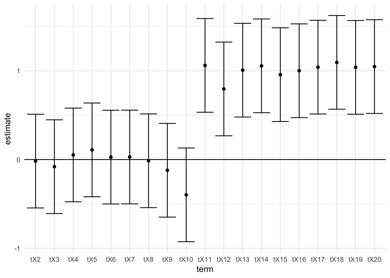

Given the dip here (evident in the ECL plot), I’ve excluded the first time period (here, t=1). Normally, one would exclude the pre-treatment period (here, t=10).

---

The triple difference

A difference-in-difference-in-differences (DDD) model allows us to study the effect of treatment on different groups. If we are concerned that our estimated treatment effect might be spurious, a common robustness test is to introduce an additional comparison group that is either untreated or (potentially) treated differently. For example, if we want to know how welfare reform influenced labor force participation, we can use a DD model that takes advantage of policy variation across states, and then use a DDD model to study how the policy has influenced single and married women differently.

As in the difference-in-differences discussion, DDD estimation is only appropriate where DD is appropriate. (Note that DDDs typically use several years of serially correlated data but ignore the resulting inconsistency of standard errors (see Bertrand, Duflo, and Mullainathan, 2004).)