Chapter 10 Regression discontinuity
General discussion
“Regression discontinuity (RD) designs for evaluating causal effects of interventions where assignment to a treatment is determined at least partly by the value of an observed covariate lying on either side of a cutoff point were first introduced by Thistlewaite and Campbell (1960). With the exception of a few unpublished theoretical papers (Goldberger, 1972a; Goldberger, 1972b), these methods did not attract much attention in the economics literature until recently. Starting in the late 1990s, there has been a growing number of studies in economics applying and extending RD methods, starting with Van der Klaauw (2002), Lee (2008), Angrist and Lavy (1999), and Black (1999). Around the same time, key theoretical and conceptual contributions, including the interpretation of estimates for fuzzy RD designs and allowing for general heterogeneity of treatment effects, were developed by Hahn, Todd, and van der Klaauw (2001).” (This is the introductory paragraph from the 2008 Imbens and Lemieux editorial, in the {}.)
Suppose you’re interested in the causal effect of a binary intervention or treatment. As illustrated nicely in Imbens and Lemieux (2008), consider a scenario where economic agents (e.g., individuals, firms, countries) are either exposed or not exposed to a treatment. Let \(Y_i(0)\) and \(Y_i(1)\) denote the pair of potential outcomes for agent \(i\): \(Y_i(0)\) is the outcome without exposure to the treatment and \(Y_i(1)\) is the outcome given exposure to the treatment. In general, we might be interested in some comparison of \(Y_i(0)\) and \(Y_i(1)\), e.g., the difference \(Y_i(1) - Y_i(0)\).
Fundamental to the empirical problem of drawing causal inference is that we never observe the pair \(Y_i(0)\) and \(Y_i(1)\) together. We therefore typically focus on average effects of the treatment, that is, averages of \(Y_i(1) - Y_i(0)\) over (sub)populations (e.g., \({\bar Y}_i(1) - {\bar Y}_i(0)\)) rather than on unit-level comparison.
For our example, let \(W_i \in \{0,1\}\) denote the treatment received, with \(W_i=1\) if unit \(i\) was exposed to the treatment, and \(W_i=0\) otherwise. The outcome observed can then be written as \[Y_i= W_i \cdot Y_i(1) + (1-W_i) \cdot Y_i(0)\] In addition to the assignment and outcome, \(W_i\) and \(Y_i\), we may also observe a vector of covariates or pre-treatment variables, denoted by \((X_i,Z_i)\), known not to have been affected by the treatment.
The basic idea behind the RD design is that the assignment of treatment is determined, either completely or partly, by the value of a predictor (the covariate \(X_i\)) being on either side of a fixed threshold. This predictor may itself be associated with the potential outcomes, but this association is assumed to be smooth, and so any discontinuity of the conditional distribution of the outcome as a function of this covariate at the cutoff value (or of a feature of this conditional distribution such as the conditional expectation) is interpreted as evidence of a causal effect of the treatment.
The design often arises from administrative decisions, where the incentives for units to participate in a program are partly limited for reasons of resource constraints, and clear transparent rules rather than discretion by administrators are used for the allocation of these incentives. Examples of such settings abound. For example, Hahn, Todd, and van der Klaauw (2001) study the effect of an anti-discrimination law that only applies to firms with at least 15 employees. In another example, Matsudaira (2007) studies the effect of a remedial summer school program that is mandatory for students who score less than some cutoff level on a test (see also Jacob and Lefgren, 2004). Access to public goods such as libraries or museums is often eased by lower prices for individuals depending on an age cutoff value (senior citizen discounts and discounts for children under some age limit). Similarly, eligibility for medical services through medicare is restricted by age (Card et al., 2004).
It is useful to distinguish between two general settings, the sharp and the fuzzy regression discontinuity designs (e.g., Trochim, 1988; Hahn, Todd, and van der Klaauw, 1999).
Sharp Regression Discontinuity (SRD)
Regression discontinuity designs are considered “sharp” when the entity faces mandatory participation in a program whenever a reference variable exceeds a specific value; if the reference variable falls below that value, the entity is ineligible for the program. (The tradition is to think of treatment falling on the right side of the cutoff. In reality, institutional knowledge will dictate where exactly the cutoff is and which group—those left or right of the cutoff—constitute the treated.) Such __sharp designs often arise from administrative decisions, where clear and transparent rules (rather than discretion by administrators) are used to allocate incentives/treatment}.
Consider the assignment \(W_i\) as a deterministic function of one of the covariates, the forcing (or running, or treatment-determining) variable, \(X\): \[W_i = 1\{ X_i \ge c \}.\] That is, all units with a covariate value of at least \(c\) are assigned to the treatment group (and participation is mandatory for these individuals), and all units with a covariate value less than \(c\) are assigned to the control group (members of this group are not eligible for the treatment). This clearly presents a problem as __there is no overlap… one cannot compare treated and untreated individuals over the range of \(x\) as one only sees difference at the \(x=6\) threshold}. This leads to the unavoidable need for extrapolation. In the SRD design, we look at the discontinuity in the conditional expectation of the outcome given the covariate to uncover an average causal effect of the treatment:
The __average treatment effect at \(c\)}: the limit of the conditional expectation of \(y\) given \(x\), as \(x\) approaches the cutoff point \(c\) from above, minus the limit of the conditional expectation of \(y\) given \(x\), as \(x\) approaches the cutoff point \(c\) from below. Equivalently, \[\tau_{SRD}=\lim_{x \downarrow c} E[Y | X=x] - \lim_{x \uparrow c} E[Y | X=x].\]
Examples:
- an anti-discrimination law applying only to firms with at least 15 employees (Hahn, Todd, and van der Klaauw, 1999)
- a mandatory remedial summer school program for students who score less than some cutoff level on a standardized test (Matsudaira, 2008; Jacob and Lefgren, 2004)
- age-based monopoly price discrimination for “children under 12” or for “seniors over 65”
- eligibility for Medicare services by age (Card, Dobkin, and Maestas, 2004)
- priority listing among toxic-waste sites by Hazard Ranking Score (Greenstone and Gallagher, 2005)
Figures 1 and 2 of Imbens and Lemieux (2008) illustrate the identification strategy in the SRD setup. “Based on artificial population values, Fig. 1 shows the conditional probability of receiving the treatment, \(Pr(W=1\mid X=1)\) against the covariate \(x\). At \(x = 6\) the probability jumps from 0 to 1. In Fig. 2, three conditional expectations are plotted. The two continuous lines (partly dashed, partly solid) in the figure are the conditional expectations of the two potential outcomes given the covariate, \(\mu_W(x)=E[Y(w) \mid X=x]\), for \(w=0,1\). These two conditional expectations are continuous functions of the covariate. Note that we can only estimate \(\mu_0(x)\) for \(x<c\) and \(\mu_1\) for \(x \ge c\).” The solid line is the conditional expectation of the observed outcome, \(E[Y \mid X=x]\), or \[E[Y \mid W =0, X=x] \cdot Pr(W=0, X=x) + E[Y \mid W =1, X=x] \cdot Pr(W=1, X=x).\]
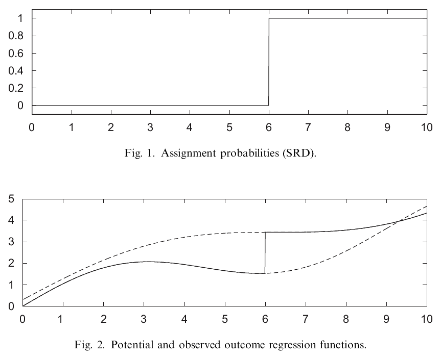
Figure 10.1: Imbens and Lemieux (J of Econometrics 2008), Fig. 1 and Fig. 2
Lee, 2008: The effect of party affiliation of a congressman/woman on congressional voting outcomes. Electoral districts where the share of the vote for a Democrat is a particular election was just under 50% are on average similar in many relevant respects to districts where the share of the Democratic vote was just over 50% but the small difference in votes leads to an immediate and big difference in the party affiliation of the elected representative. In this case, the party affiliation always jumps at 50%, making this an SRD design. Lee considers the “incumbency effect,” being interested in the probability that Democrats win the subsequent election, comparing districts where the Democrats won the previous election with just over 50% of the popular vote with districts where the Democrats lost the previous election with just under 50% of the vote.
Chay and Greenstone, 2004: Compare counties that are in and out of attainment with Clean Air Act standards (just above and just below the requirements).
Fuzzy Regression Discontinuity (FRD)
As an alternative to the above, suppose that treatment is not discontinuously “forced” on subjects at \(x_i = c\), but, rather, is more likely at \(c\). When the probability of receiving treatment does not change sharply from 0 to 1 as \(x\) crosses threshold \(c\), the SRD is no longer appropriate. (Selection may depend upon observables and upon factors unobserved by the investigator.) Instead of a sharp 0 to 1 change in probability, for example, there can often be a discrete (but smaller) jump in treatment probability as the threshold is passed:
- Participation in summer school remedial programs can be “strongly recommended” for students with scores less than \(c\), where students with higher scores are eligible, but not exhorted to attend.
- Attendance is not compulsory for students with lower scores, but pressure is positive and gets higher with greater shortfalls compared to the threshold score \(c\).
Such examples imply that \[\lim_{x \downarrow c} Pr(W_i = 1 | X_i=x) \ne \lim_{x \uparrow c} Pr(W_i = 1 | X_i=x).\]
In these models, the “average treatment effect” at \(c\) is calculated as the difference in the outcome variable as \(x\) approaches \(c\) from above and below, divided by the difference in the probability of treatment as \(x\) approaches \(c\) from above and below: \[\tau_{FRD}=\frac{\lim_{x \downarrow c} E[Y | X=x] - \lim_{x \uparrow c} E[Y | X=x]}{\lim_{x \downarrow c} Pr[W | X_i=x] - \lim_{x \uparrow c} Pr[W | X_i=x]}\]
Here, the probability of being “treated” may differ with \(x\) throughout the range of \(x\), rather than shifting simply from zero to one when \(x\) passes the critical threshold of 6. There are still two profiles for \(y\) as a function of \(x\) (either without treatment or with treatment). However, below \(c\) we no longer see the “true” expected value for \(y\) given \(x\) without treatment. Likewise, above \(c\) we no longer see the “true” expected value for \(y\) given \(x\) with treatment. We see a mix.
In Fig. 3 of Imbens and Lemieux (2008) they plot the conditional probability of receiving the treatment for a FRD design. “As in the SRD design, this probability still jumps at \(x=6\), but now by an amount less than 1. Fig. 4 presents the expectation of the potential outcomes given the covariate and the treatment, \(E[Y(w)\mid W=w,X=x]\), represented by the dashed lines, as well as the conditional expectation of the observed outcome given the covariate (solid line),” \(E[Y \mid X=x]\), or \[E[Y(0) \mid W =0, X=x] \cdot Pr(W =0, X=x) + E[Y(1) \mid W =1, X=x] \cdot Pr(W =1, X=x).\]
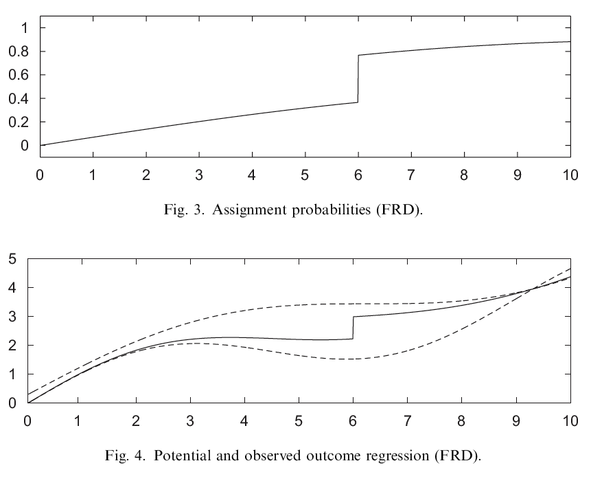
Figure 10.2: Imbens and Lemieux (J of Econometrics 2008) Fig. 3 and Fig. 4
Example of FRD design: van der Klaauw (2002), “Estimating the effect of financial aid on acceptance of college admission offers.” \(X\) is a numerical score assigned to each applicant based on their application information (e.g., SAT scores, grades). Applicants are divided into groups based on their admissions index score. Suppose there were just two categories and a single cutoff point \(c\).Scoring above \(c\) puts the applicant in a higher category and enhances their chance of an offer of financial aid. Having a score below \(c\) means a lower chance of financial aid. On the one hand, an offer of aid makes the college more attractive to a potential student (and this is the “policy” effect of interest to the college). However, a student who gets a generous offer of financial aid is likely to have other good offers as well. What makes this an FRD design is that the index score is not the sole determinant of financial aid offers, since there is non-quantitative information in the admissions essay and the letters of reference. Nevertheless, there is a clear discontinuity in the probability of an aid offer at the cutoff point \(c\)."
In closing, do note that the “fuzzy” modifier is somewhat misleading, as the underlying discontinuity must be “sharp” in both SRD and FRD designs.
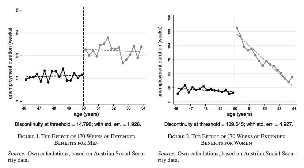
Figure 10.3: Lalive (AER 2007), Fig. 1 and Fig. 2
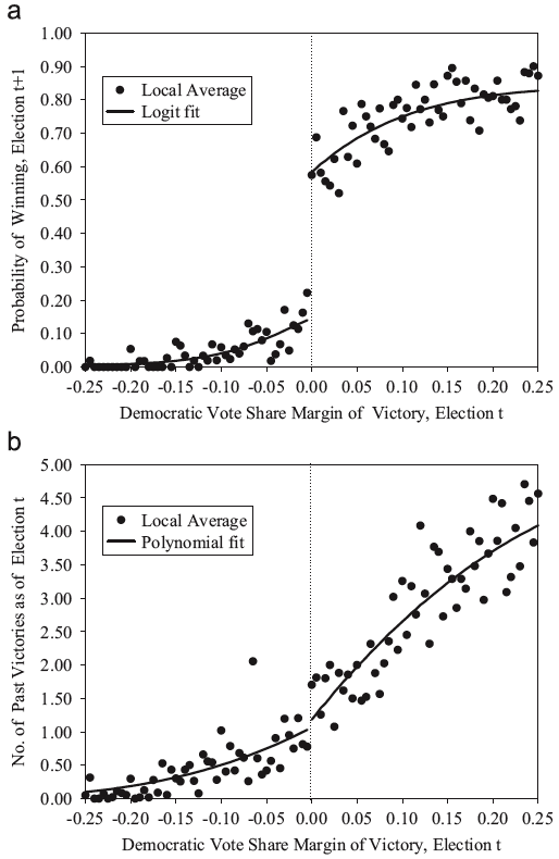
Figure 10.4: Lee (J of Econometrics 2008) Fig. 1 and Fig. 2
Fig. a: Candidate’s probability of winning election \(t+1\), by margin of victory in election \(t\): local averages and parametric fit
Fig. b: Candidate’s accumulated number of past election victories, by margin of victory in election \(t\): local averages and parametric fit.
Other RD issues
RD Presentation
RD has a visual appeal that is lacking in many other econometric approaches. As such, employing figures to convince the reader of your argument should be considered. See Imbens and Lemieux (2008) for suggestions about what should be included in RD papers.
- \(W_i\) by \(x_i\): Plotting a binary treatment against \(x_i\) will assist in justifying the use of SRD over FRD.
- \(Y_i\) by \(x_i\): Motivation is always a key part of presentation. This will motivate the RD strategy if outcomes change dramatically at \(x_i = c\).
- \(z_i\) by \(x_i\): Useful for specification testing.
Specification testing:
- Make sure that there is a zero average effect on other outcomes known to not have been affected by the treatment. (If effect does happen where it might, make sure it does not happen where it shouldn’t.)
- Tests of continuity of the density (i.e., no jumps in the forcing variable, just the program participation probability in response to increases in its level)
- Estimate “jumps” at points where there should be no jumps (i.e., test for treatment effects in setting where it is known that the effect should be zero).
RD Bandwith
The neighbourhood around \(c\) — that is, the bandwidth — is the econometrician’s (referee’s?) choice. Imbens and Lemieux propose a bandwidth chosen by cross-validation. (Cross-validation is one of several approaches to estimating how well a model that employs some “training” data is going to perform on future as-yet-unseen data — like out-of-sample prediction, for example.) Intuitively, consider that increasing bandwidth \(h\) purchases precision at the cost of relevance. In essence, the econometrician must have sufficient sample size to estimate the conditional means on both sides of the discontinuity, but does not want to confound estimates with distant or increasingly irrelevant observations.
“Guide to Practice”
Imbens and Lemieux (J of Econometrics, 2008) offers the following, as part of their “guide to practice.” (Note: Like most things… best-practice guides have a shelf life. For example, we used to allow for clustering on the running variable, which was brought into question )
Case 1: SRD designs
- Graph the data by computing the average value of the outcome variable over a set of bins. The binwidth has to be large enough to have a sufficient amount of precision so that the plot looks smooth on either side of the cutoff value, but at the same time small enough to make the jump around the cutoff value clear.
- Estimate the treatment effect by running linear regressions on both sides of the cutoff point. Since we propose to use a rectangular kernel, these are just standard regression estimates within a bin of width \(h\) on both sides of the cutoff point.
- Standard errors can be computed using standard least square methods (robust standard errors).
- The optimal bandwidth can be chosen using cross-validation methods.
- Standard errors can be computed using standard least square methods (robust standard errors).
- The robustness of the results should be assessed by employing various specification tests.
- Looking at possible jumps in the value of other covariates at the cutoff point.
- Testing for possible discontinuities in the conditional density of the forcing variable.
- Determining whether the average outcome is discontinuous at other values of the forcing variable.
- Using various values of the bandwidth, with and without other available covariates.
Case 2: FRD designs
A number of issues arise in the case of FRD designs in addition to those mentioned above.
- Graph the average outcomes over a set of bins as in the case of SRD, but also graph the probability of treatment.
- Estimate the treatment effect using 2SLS, which is numerically equivalent to computing the ratio in the estimate of the jump (at the cutoff point) in the outcome variable over the jump in the treatment variable.
- Standard errors can be computed using the usual (robust) 2SLS standard errors, though a plug-in approach can also be used instead.
- The optimal bandwidth can again be chosen using a modified cross-validation procedure.
- The robustness of the results can be assessed using the various specification tests mentioned in the case of SRD designs. In addition, FRD estimates of the treatment effect can be compared to standard estimates based on unconfoundedness.
RD in Stata
In the simplest case, assignment to treatment depends on a variable \(Z\) being above a cutoff \(Z_0\). Frequently, \(Z\) is defined so that \(Z_0=0\). In this case, treatment is 1 for \(Z \ge 0\) and \(0\) for \(Z<0\), and we estimate local linear regressions on both sides of the cutoff to obtain estimates of the outcome at \(Z=0\). The difference between the two estimates (for the samples where \(Z \ge 0\) and where \(Z<0\)) is the estimated effect of treatment.
For example, having a Democratic representative in the US Congress may be considered a treatment applied to a Congressional district, and the assignment variable \(Z\) is the vote share garnered by the Democratic candidate. At \(Z=50\%\), the probability of this kind of treatment jumps from zero to one. Suppose we are interested in the effect a Democratic representative has on the federal spending within a Congressional district.
Method 1
rd estimates local linear regressions on both sides of the cutoff. Using the dataset votex.dta. Be sure to install the rd command. This is available from http://ideas.repec.org/c/boc/bocode/s456888.html, and locpoly.
ssc inst rd, replace
net get rd
use votex if i==1
* d = Dem vote share minus .5
* lne = Log fed expenditure in district
*  rd [varlist] [if] [in] [weight] [, options]
* varlist has form: outcomevar [treatmentvar] assignmentvar
rd lne d, gr mbw(100) k(rec) adoonly
rd lne d, gr mbw(100) k(rec) adoonly line(`"xla(-.2 "Repub" 0 .3 "Democ", noticks)"')
rd lne d, gr ddens adoonly
bs: rd lne d, x(pop-vet) adoonly
Method 2
Assume that the assignment variable \(Z\) is called share and ranges from 1 to 99 with an assignment cutoff at 50. (For example, submit ge share = round((d+.5)*100,1) if using votex.dta.)
prog discont, rclass
version 8.2
cap drop z f0 f1
g z=\_n in 1/99
locpoly `1' share if share<50, gen(f0) at(z) nogr tri w(2) d(1) ep
locpoly `1' share if share>=50, gen(f1) at(z) nogr tri w(2) d(1) ep
return scalar d=`f1'[50]-`f0'[50]
end
bootstrap r(d), reps(1000): discont lne
The computation of the difference in outcomes \(y^+ - y^-\) is obtained by replacing \(x\) with \(y\) in the above. The local Wald estimator of LATE is then \[\frac{y^+ - y^-}{x^+ - x^-},\] which quantity can also be computed in a program and bootstrapped. Imbens and Lemieux (2007) also provide analytic standard error formulae.
Note that bootstrap performs bootstrap estimation. Typing bootstrap exp_list, reps(\#): command executes command multiple times, bootstrapping the statistics in exp_list by re-sampling observations (with replacement) from the data in memory # times. This is commonly referred to as the nonparametric bootstrap method.
Method 3
This program accepts the cutoff in \(X\) that triggers treatment:
program regdis, rclass
version 10.1
syntax [varlist(min=2 max=2)] [, cut(real 0) ]
tokenize `varlist'
tempvar z p0 p1
qui g `z'=`cut' in 1
local opt "deg(1) at(`z') k(tri) nogr"
lpoly `1' `2' if `2'<`cut', gen(`p0') se(`se0') `opt'
lpoly `1' `2' if `2'>=`cut', gen(`p1') se(`se1') `opt'
if `p1'[1]-`p0'[1] > 0 {
    return scalar d=`p1'[1]-`p0'[1]
    di as txt "Estimate: " as res `p1'[1]-`p0'[1]
}
else {
    return scalar d=`p0'[1]-`p1'[1]
    di as txt "Estimate: " as res `p0'[1]-`p1'[1]
}
end

regdis y x, cut(10)
bs r(d): regdis y x, cut(10)
RD in R
Simulated
Note that the simulation below accommodated a FRD design.
library(MASS)
mu <- c(0, 0)
sigma <- matrix(c(1, 0.7, 0.7, 1), ncol = 2)

set.seed(100)
d <- as.data.frame(mvrnorm(1e3, mu, sigma))

# Create treatment variable
d$treat <- ifelse(d$V1 <= 0, 1, 0)

# Introduce fuzziness
d$treat[d$treat == 1][sample(100)] <- 0
d$treat[d$treat == 0][sample(100)] <- 1

# Treatment effect
d$V2[d$treat == 1] <- d$V2[d$treat == 1] + 1

# Add grouping factor
d$group <- gl(9, 1e3/9)library(RColorBrewer)
pal <- brewer.pal(5, "RdBu")
# Fit model
m <- lm(V2 ~ V1 + treat, data = d)
ggplot(d, aes(x = V1, y = V2, color = factor(treat, labels = c('Control', 'Treatment')))) +
geom_point(shape = 21) +
scale_color_brewer(NULL, type = 'qual', palette = 6) +
geom_vline(aes(xintercept = 0), color = 'grey', size = 1, linetype = 'dashed') +
geom_segment(data = data.frame(t(predict(m, data.frame(V1 = c(-3, 0), treat = 1)))),
aes(x = -3, xend = 0, y = X1, yend = X2), color = pal[4], size = 1) +
geom_segment(data = data.frame(t(predict(m, data.frame(V1 = c(0, 4), treat = 0)))),
aes(x = 0, xend = 4, y = X1, yend = X2), color = pal[2], size = 1) 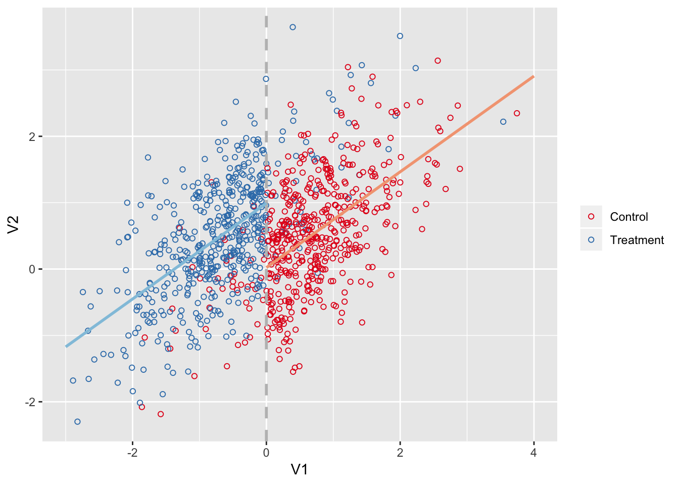
Example
See Carpenter and Dobkin (2009, 2011) for the original analysis. Also, see Mastering Metrics by Angrist and Pischke for additional material.
library(AER)
library(foreign)
mlda <- read.dta("http://masteringmetrics.com/wp-content/uploads/2015/01/AEJfigs.dta")
library(rdd)
#We then create a dummy for age over 21.
mlda$over21 = mlda$agecell>=21
attach(mlda)
#We then fit two models, the second has a quadratic age term.
fit=lm(all~agecell+over21)
fit2=lm(all~agecell+I(agecell^2)+over21)
#We plot the two models fit and fit2, using predicted values.
predfit = predict(fit, mlda)
predfit2=predict(fit2,mlda)
# plotting fit
plot(predfit~agecell,type="l",ylim=range(85,110),
     col="red",lwd=2, xlab="Age",
     ylab= "Death rate from all causes (per 100,000)")
# adding fit2
points(predfit2~agecell,type="l",col="blue")
# adding the data points
points(all~agecell)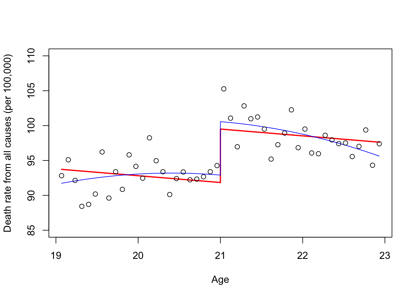
# We can plot the data and use a loess smoother for age below and above 21.
ggplot(mlda, aes(x = agecell, y = all,colour=over21)) +
  geom_point() +
  ylim(80,115) +
  stat_smooth(method = loess)
Note that there is also a specialized package called rdd for regression discontinuity analysis.
McCrary tests
McCrary (J of Econometrics 2008) introduces a density test for manipulation of the running variable in the RDD. The intuition is that a discontinuity in the density of the running variable at the threshold for treatment must be explained, and a reasonable explanation is that agents were able to manipulate their treatment status. To the extent they were, we worry that is is non-random (wrt outcomes) and thereby intriducing bias in the RDD-estimated treatment.
library(rdd)
#No discontinuity
x<-runif(1000,-1,1)
DCdensity(x,0)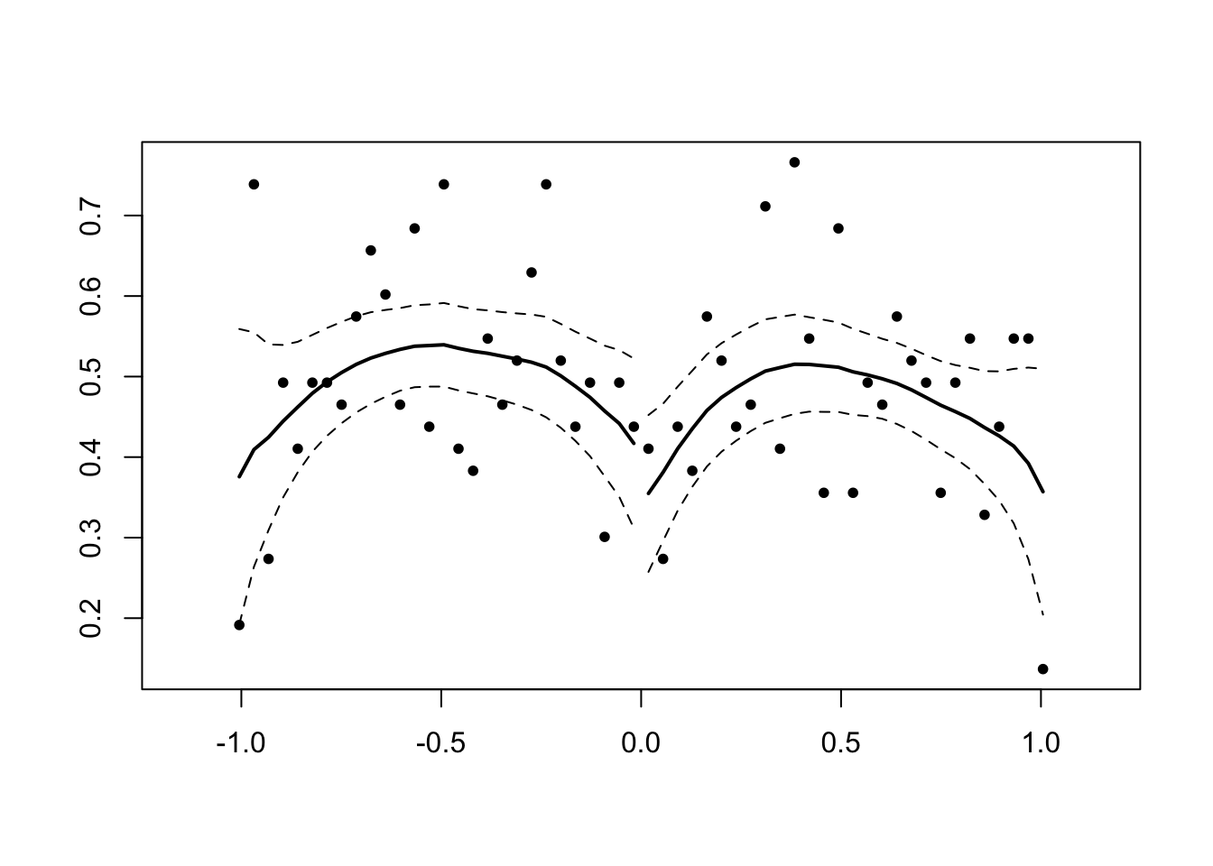
## [1] 0.5176919#Discontinuity
x<-runif(1000,-1,1)
x<-x+1*(runif(1000,-1,1)>0&x<0)
DCdensity(x,0)
## [1] 1.81302e-06Donut RD
Almond, Doyle, Kowalski, and Williams (QJE 2010) use a regression discontinuity design to argue that 1-year infant mortality decreases by approximately one percentage point as birth weight crosses the 1,500g “very low birth weight (VLBW)” threshold from above. Relative to mean 1-year mortality of 5.5% just above 1,500g, the implied treatment effect is sizable, suggesting large returns to promoting the types of medical interventions triggered by VLBW classification. Given the importance of the research question, Barreca, Guldi, Lindo, and Waddell (QJE 2011) and Barreca, Lindo, and Waddell (EcInquiry 2016) revisit the research question, developing what is now known as Donut-RD.
Barreca, Guldi, Lindo, and Waddell (QJE 2011): demonstrating the sensitivity of the ADKW result to the removal of observations at the RD threshold. 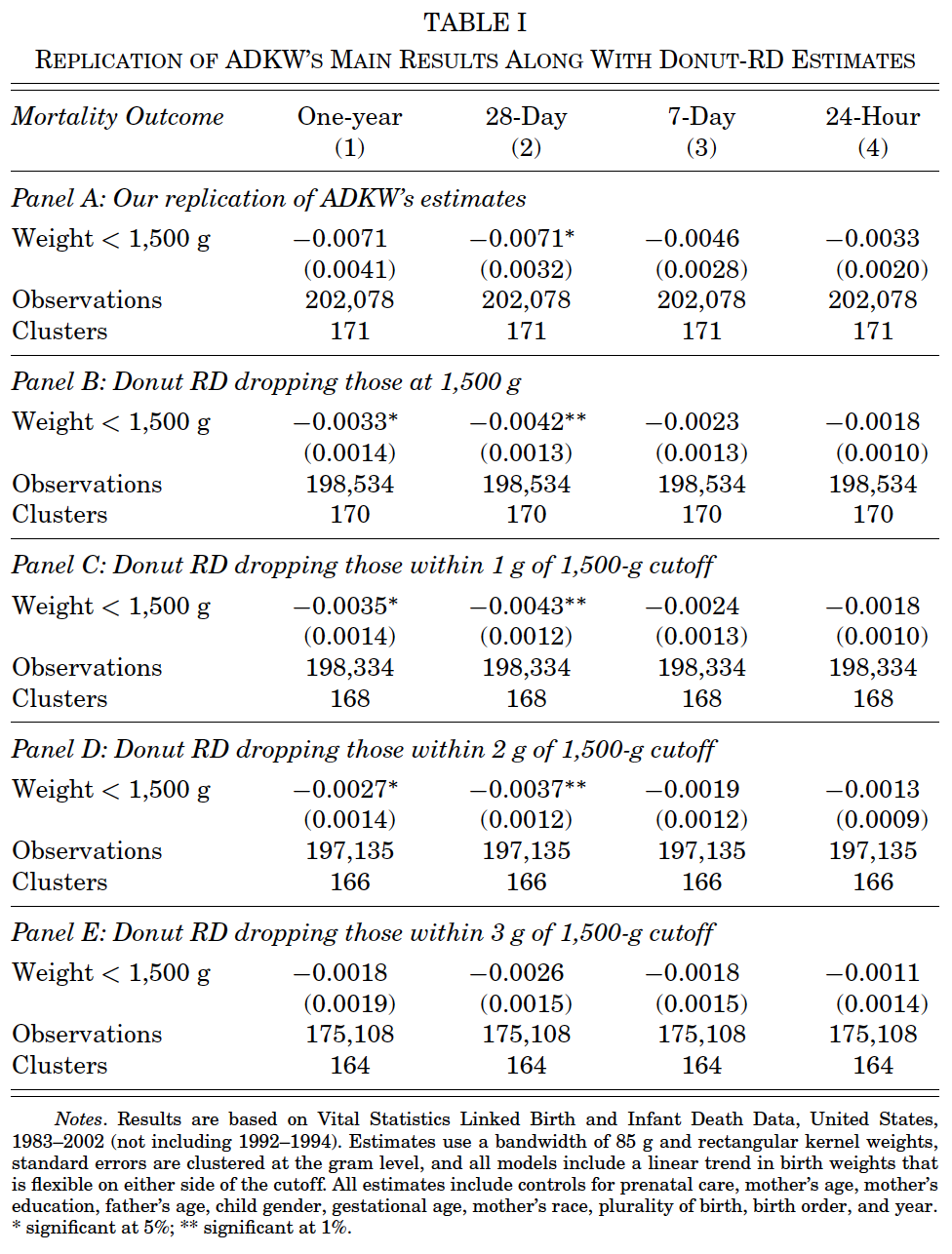
Barreca, Guldi, Lindo, and Waddell (QJE 2011): demonstrating the non-random sorting onto 100-gram and 1-ounce multiples. 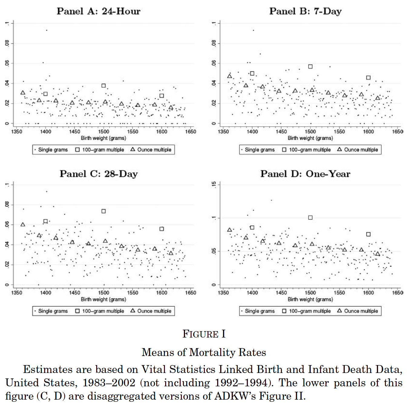
Barreca, Lindo, and Waddell (EcInquiry 2016): demonstrating ADKW-like results at every 100-gram multiple, in the absence of treatment. 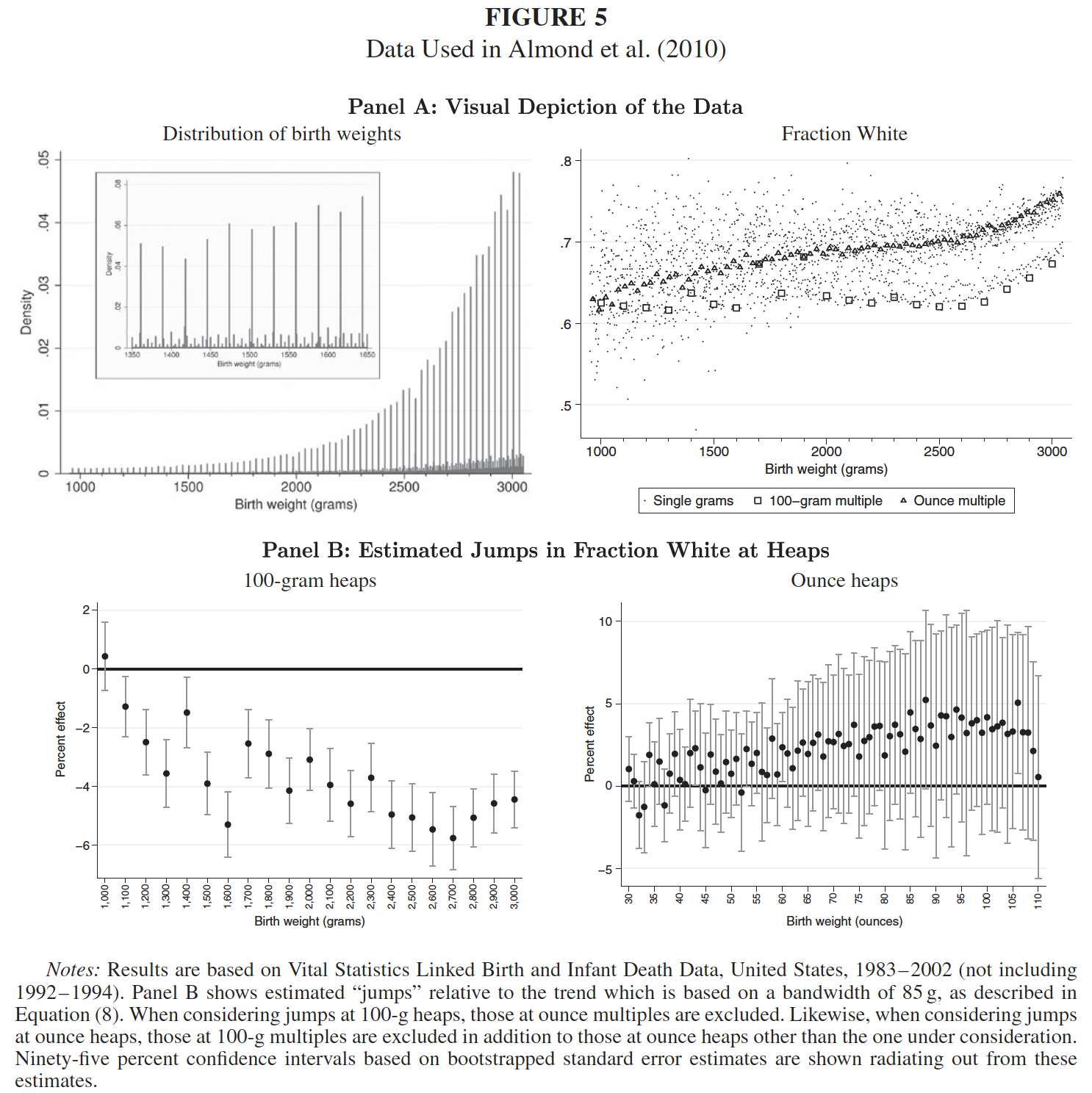
Barreca, Lindo, and Waddell (EcInquiry 2016): patterns of estimated discontinuities across samples 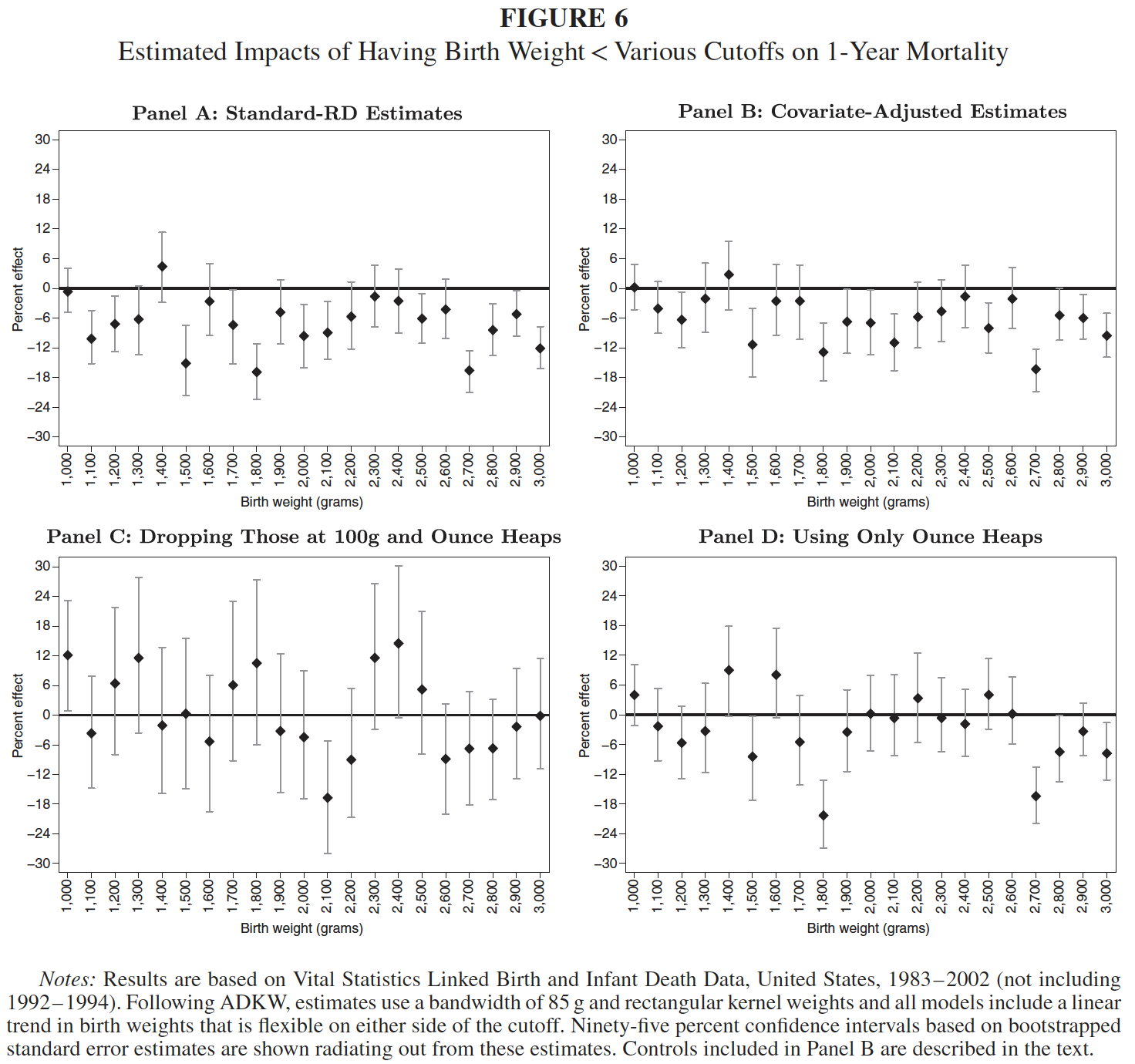
Barreca, Lindo, and Waddell (EcInquiry 2016): Non-random sorting in birth weight 
Literature
Other considerations from the literature include: Thistlewaite and Campbell (1960), Goldberger (1972a, 1972b), Cain (1975), Hahn, Todd, and van der Klaauw (2001), van der Klaauw (2002, 2008), Lee, Moretti, and Butler (2004), Chapter 25 of Cameron and Trivedi (2005).