Chapter 13 Standard-error estimation
library(mvtnorm)
library(multiwayvcov)
library(dplyr)
library(ggplot2)
library(arm)
library(clusterSEs)
13.1 Simulations of Linear Regression
Setting Up Simulations
First, let us create a function to create data. Here we suppose a simple regression model: \[y_i \backsim N(~\beta_0+\beta_1x_i~,~\sigma^2~)\]
In the function, intra-cluster correlation will be controlled by rho (\(\rho\)). When \(\rho=1\), all units within a cluster are considered to be identical, and the effective sample size is reduced to the number of clusters. When \(\rho=0\), there is no correlation of units within a cluster, and all observations are considered to be independent of each other.
gen_cluster <- function(param = c(.1, .5), n = 1000, n_cluster = 50, rho = .5) {
    # Function to generate clustered data
    # Required package: mvtnorm

    # individual level
    Sigma_i <- matrix(c(1, 0, 0, 1 - rho), ncol = 2)
    values_i <- rmvnorm(n = n, sigma = Sigma_i)

    # cluster level
    cluster_name <- rep(1:n_cluster, each = n / n_cluster)
    Sigma_cl <- matrix(c(1, 0, 0, rho), ncol = 2)
    values_cl <- rmvnorm(n = n_cluster, sigma = Sigma_cl)

    # predictor var consists of individual- and cluster-level components
    x <- values_i[ , 1] + rep(values_cl[ , 1], each = n / n_cluster)

    # error consists of individual- and cluster-level components
    error <- values_i[ , 2] + rep(values_cl[ , 2], each = n / n_cluster)

    # data generating process
    y <- param[1] + param[2]*x + error

    df <- data.frame(x, y, cluster = cluster_name)
    return(df)
}
Next, let us make some functions to run simulations.
# Simulate a dataset with clusters and fit OLS
# Calculate cluster-robust SE when cluster_robust = TRUE
cluster_sim <- function(param = c(.1, .5), n = 1000, n_cluster = 50,
                            rho = .5, cluster_robust = FALSE) {
    # Required packages: mvtnorm, multiwayvcov
    df <- gen_cluster(param = param, n = n , n_cluster = n_cluster, rho = rho)
    fit <- lm(y ~ x, data = df)
    b1 <- coef(fit)[2]
    if (!cluster_robust) {
        Sigma <- vcov(fit)
        se <- sqrt(diag(Sigma)[2])
        b1_ci95 <- confint(fit)[2, ]
    } else { # cluster-robust SE
        Sigma <- cluster.vcov(fit, ~ cluster)
        se <- sqrt(diag(Sigma)[2])
        t_critical <- qt(.025, df = n - 2, lower.tail = FALSE)
        lower <- b1 - t_critical*se
        upper <- b1 + t_critical*se
        b1_ci95 <- c(lower, upper)
    }
    return(c(b1, se, b1_ci95))
}

# Function to iterate the simulation. A data frame is returned.
run_cluster_sim <- function(n_sims = 1000, param = c(.1, .5), n = 1000,
                            n_cluster = 50, rho = .5, cluster_robust = FALSE) {
    # Required packages: mvtnorm, multiwayvcov, dplyr
    df <- replicate(n_sims, cluster_sim(param = param, n = n, rho = rho,
                                        n_cluster = n_cluster,
                                        cluster_robust = cluster_robust))
    df <- as.data.frame(t(df))
    names(df) <- c('b1', 'se_b1', 'ci95_lower', 'ci95_upper')
    df <- df %>%
        mutate(id = 1:dplyr::n(),
        param_caught = ci95_lower <= param[2] & ci95_upper >= param[2])
    return(df)
}
Data without Clusters
First, we will run simulations of data with no cluster (\(\rho=0\)). Here, we set \(\beta_0=0.4\) and \(\beta_1=0\). Setting the significance level at 5%, we should incorrectly reject the null \(\beta_1=0\) in about five percent of the simulations.
sim_params <- c(.4, 0)   # beta1 = 0: no effect of x on y
sim_nocluster <- run_cluster_sim(n_sims = 10000, param = sim_params, rho = 0)
hist_nocluster <- ggplot(sim_nocluster, aes(b1)) +
    geom_histogram(color = 'black', binwidth=.005) +
    geom_vline(xintercept = sim_params[2], color = 'red')
print(hist_nocluster)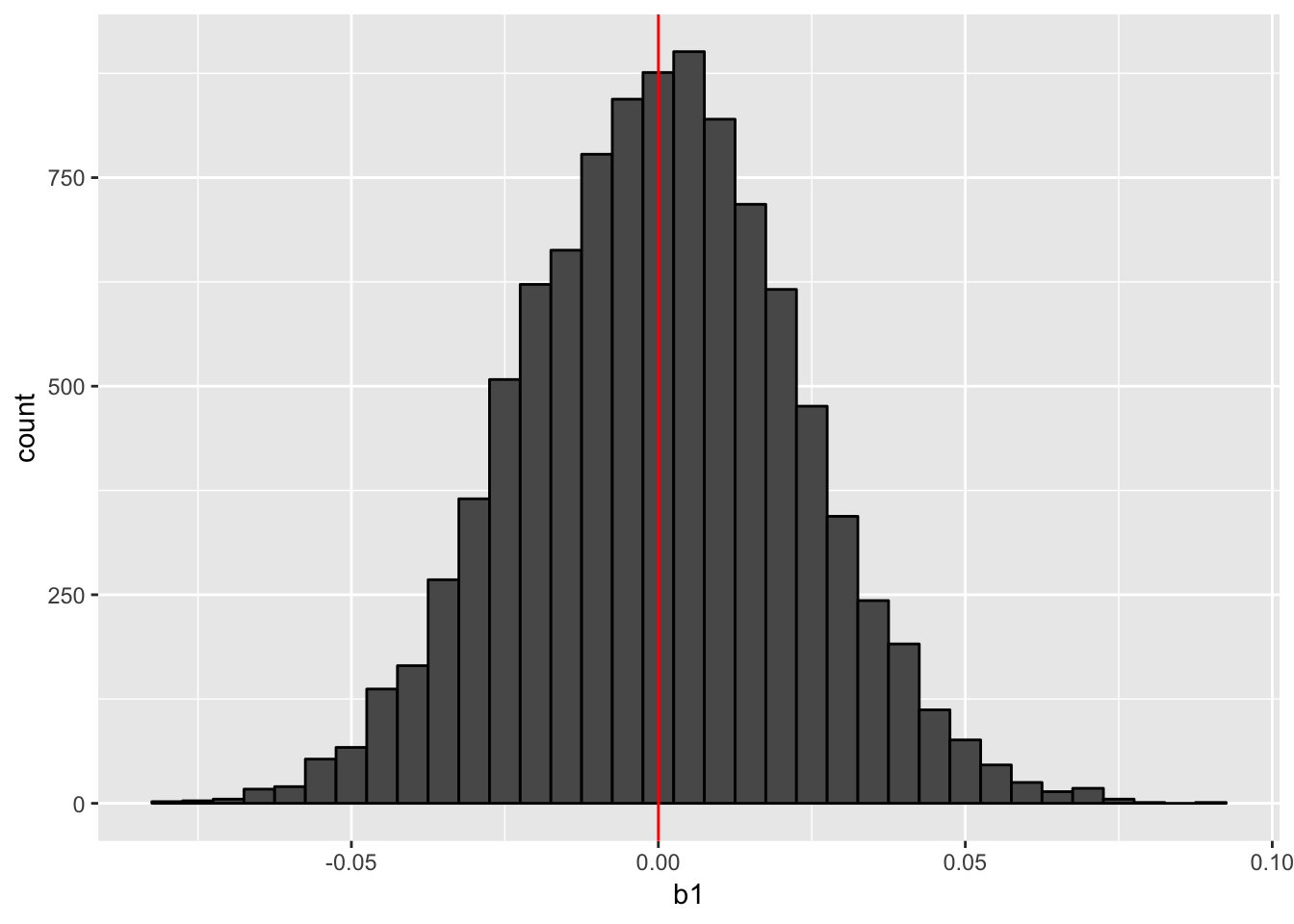
As the histogram above shows, we can estimate the value of \(\beta_1\) correctly on average. Let’s check the confidence intervals (CIs).
ci95_nocluster <- ggplot(sample_n(sim_nocluster, 100),
                         aes(x = reorder(id, b1), y = b1,
                             ymin = ci95_lower, ymax = ci95_upper,
                             color = param_caught)) +
    geom_hline(yintercept = sim_params[2], linetype = 'dashed') +
    geom_pointrange() +
    labs(x = 'sim ID', y = 'b1', title = 'Randomly Chosen 100 95% CIs') +
    scale_color_discrete(name = 'True param value', labels = c('missed', 'hit'))
print(ci95_nocluster)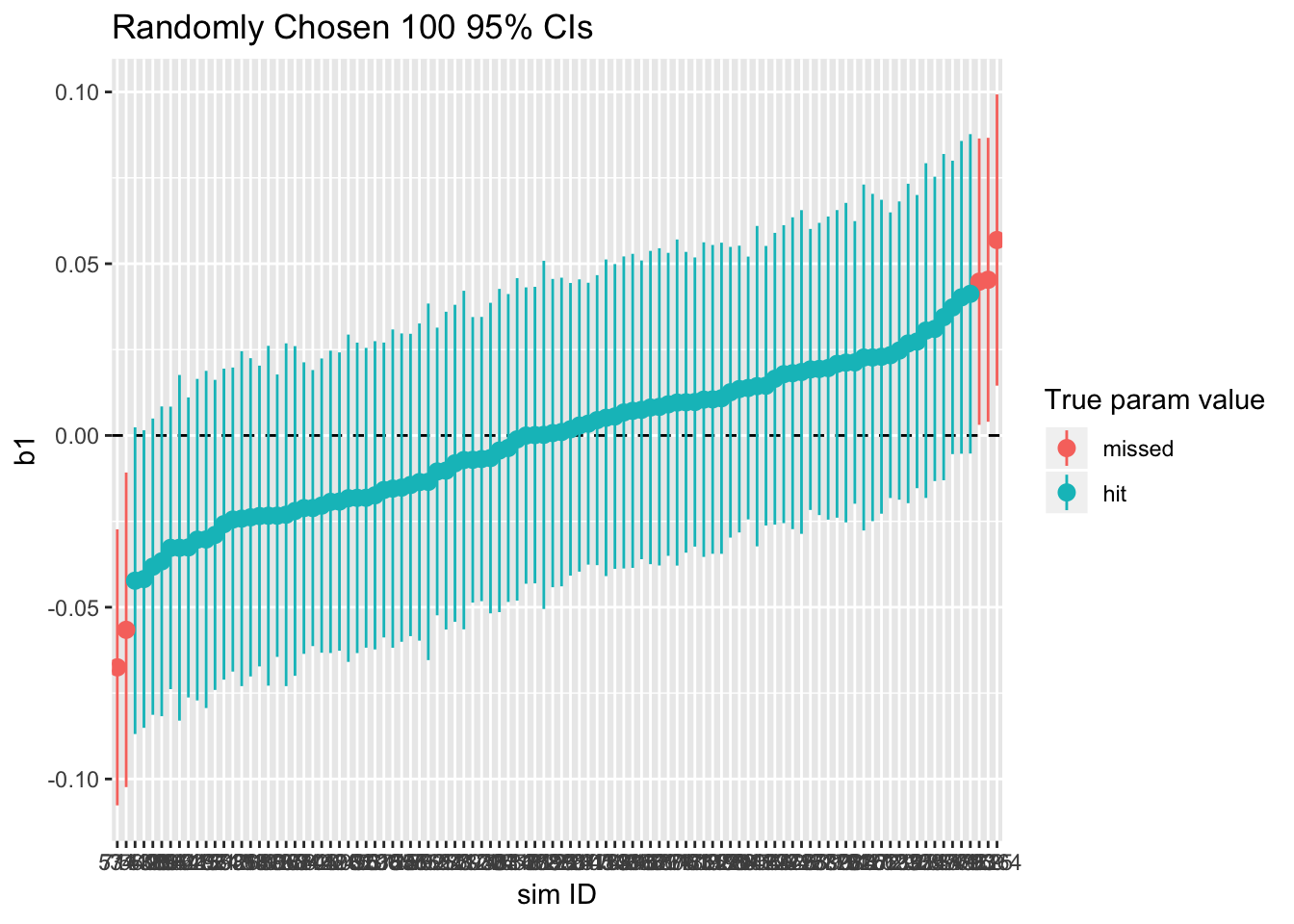
sim_nocluster %>% summarize(type1_error = 1 - sum(param_caught)/n())## type1_error
## 1 0.0501As shown, about 95% of the 95%-confidence intervals catch the true value of \(\beta_1\), which is zero. In other words, we incorrectly reject the null hypothesis about 5% of the time. This isn’t a problem, given that the rate of Type I error is close to the significance level.
Data with Clusters
Now, let us simulate data with clusters. Fist, we will fit the OLS to the clustered data.
sim_params <- c(.4, 0)   # beta1 = 0: no effect of x on y
sim_cluster_ols <- run_cluster_sim(n_sims = 10000, param = sim_params)
hist_cluster_ols <- hist_nocluster %+% sim_cluster_ols
print(hist_cluster_ols)
As this histogram shows, the point estimate is not biased; we can correctly estimate the slope on average.
How about CIs?
ci95_cluster_ols <- ci95_nocluster %+% sample_n(sim_cluster_ols, 100)
print(ci95_cluster_ols)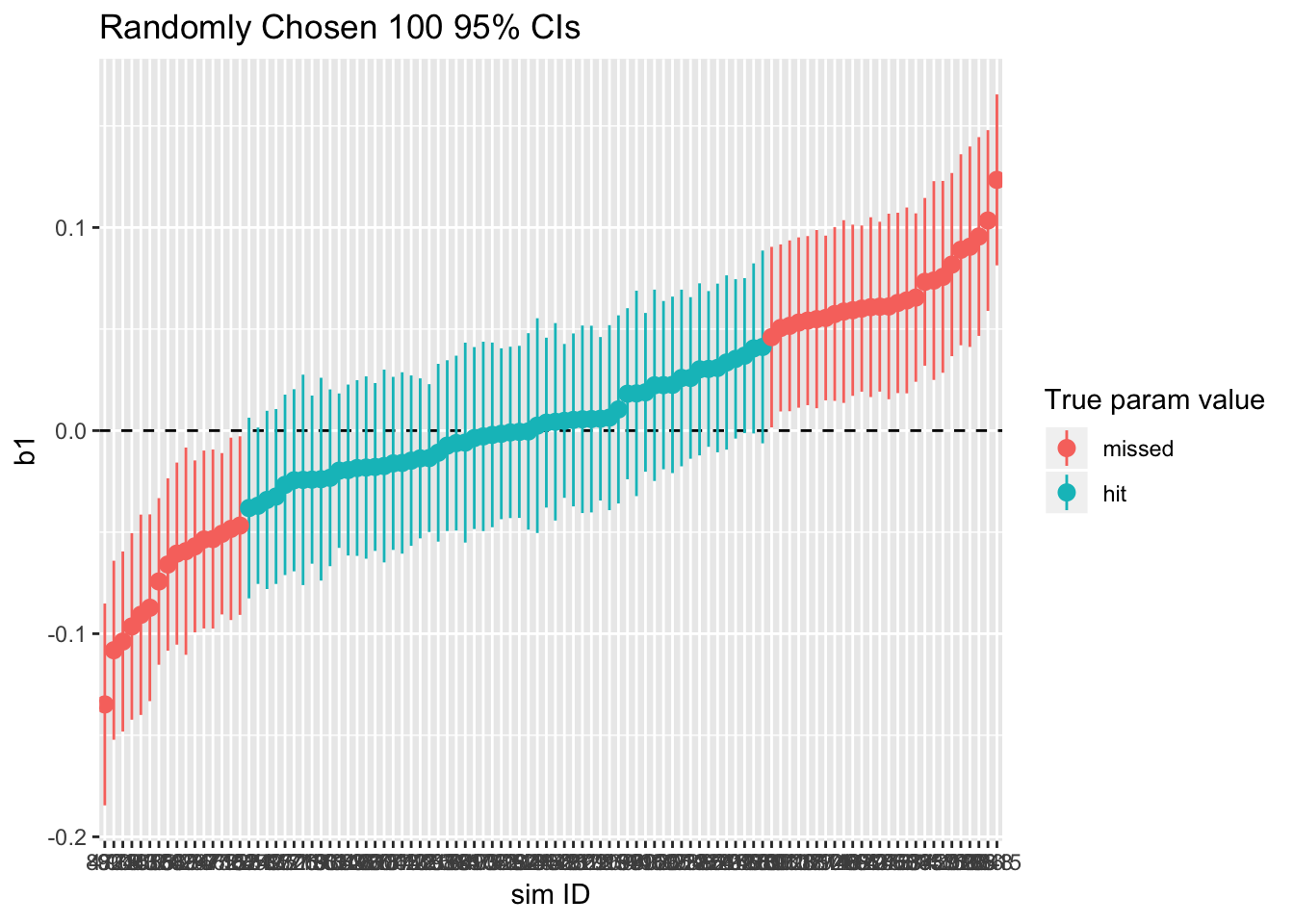
sim_cluster_ols %>% summarize(type1_error = 1 - sum(param_caught)/n())## type1_error
## 1 0.4178As shown, more than 5% of the confidence intervals miss the true values, which means that we reject the null more than 5% of the time. In other words, if we analyze clustered-data using OLS, we might (incorrectly) reject the null hypothesis more than we should. In this case, it is due to having underestimated the standard error. (This can go the other way, too, if \(\rho < 0\).)
To avoid over-reporting of “significant” results, we need to calculate cluster-robust standard errors. We can get cluster-robust var-cov by multiwayvcov::cluster.vcov() as defined in cluster_sim() above.
sim_params <- c(.4, 0) # beta1 = 0: no effect of x on y
sim_cluster_robust <- run_cluster_sim(n_sims = 10000, param = sim_params,
cluster_robust = TRUE)
hist_cluster_robust <- hist_nocluster %+% sim_cluster_ols
print(hist_cluster_robust)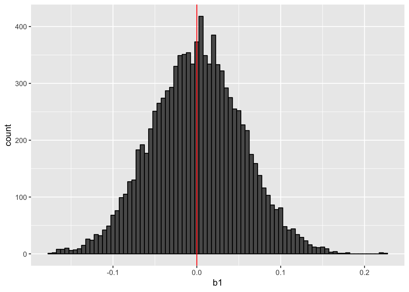 When we calculate cluster-robust SEs, we use the OLS-estimated coefficient. So this histogram is similar (identical if the same datasets were used) to the previous histogram.
Now, let us examine the CIs.
ci95_cluster_robust <- ci95_nocluster %+% sample_n(sim_cluster_robust, 100)
print(ci95_cluster_robust)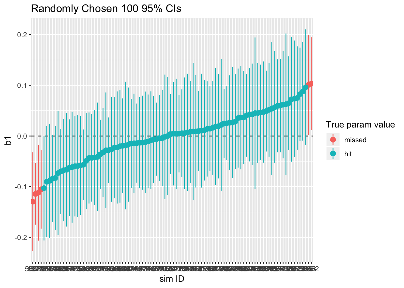
sim_cluster_robust %>% summarize(type1_error = 1 - sum(param_caught)/n())## type1_error
## 1 0.0662As shown, the rate of Type I error has decreased. This is because the cluster-robust standard errors are smaller than the standard error calculated without considering the cluster structure.
We should calculate cluster-robust standard errors when we suspect the data are clustered. Or, we should always calculate cluster-robust SEs unless we are theoretically convinced that there is no clustering in the data.
To get cluster-robust CIs more easily with cluster-bootstrap variance-covariance matrix estimates, we can use clusterSEs::cluster.bs.glm.
df_test <- gen_cluster(param = c(.4, 0))
fit_ols <- lm(y ~ x, data = df_test)
display(fit_ols)
## lm(formula = y ~ x, data = df_test)
## coef.est coef.se
## (Intercept) 0.44 0.03
## x 0.12 0.02
## ---
## n = 1000, k = 2
## residual sd = 1.05, R-Squared = 0.02confint(fit_ols)## 2.5 % 97.5 %
## (Intercept) 0.37943827 0.5098994
## x 0.06832716 0.1661302# same estimates using glm to be passed to cluster.bs.glm
fit_glm <- glm(y ~ x, data = df_test, family = gaussian(link = 'identity'))
display(fit_glm)## glm(formula = y ~ x, family = gaussian(link = "identity"), data = df_test)
## coef.est coef.se
## (Intercept) 0.44 0.03
## x 0.12 0.02
## ---
## n = 1000, k = 2
## residual deviance = 1101.2, null deviance = 1125.6 (difference = 24.4)
## overdispersion parameter = 1.1
## residual sd is sqrt(overdispersion) = 1.05confint(fit_glm)## Waiting for profiling to be done...## 2.5 % 97.5 %
## (Intercept) 0.37951738 0.5098203
## x 0.06838647 0.1660708# cluster-bootstrap CI
fit_robust <- cluster.bs.glm(fit_glm, dat = df_test, cluster = ~ cluster,
boot.reps = 1000, prog.bar = FALSE)##
## Cluster Bootstrap p-values:
##
## variable name cluster bootstrap p-value
## (Intercept) 0
## x 0.035
##
## Confidence Intervals (derived from bootstrapped t-statistics):
##
## variable name CI lower CI higher
## (Intercept) 0.215110904555314 0.674226788915819
## x 0.0143961685411534 0.220061143905432Again, in this example, the cluster-robust CI is much wider than the OLS CI.
Cluster-Robust SE, Fixed Effects, or Random Effects Models
Though the clustered-robust SEs correct the standard errors in linear regression, the cluster structure isn’t taken into account when the coefficients are estimated. What will we get if we consider the cluster structure when estimating the coefficients?
Let us think and simulate two other estimation methods as well as OLS and cluster-robust SE.
- Fixed effect model: cluster-specific fixed effects
- Random effects model: explicitly consider the two-level structure
- First level: individual units (observations)
- Second level: clusters
We can fit RE models by lme4::lmer() (see Bates et al. 2014).
To compare different models, define the function to simulate a dataset and analyze it by four different models (strictly speaking, three models and four different SEs).
sim_4models <- function(param = c(.1, .5), n = 1000, rho = .5, n_cluster = 50) {
    # Required packages: mvtnorm, multiwaycov, lme4,
    df <- gen_cluster(param = param, n = n , n_cluster = n_cluster, rho = rho)

    # Fit three different models
    fit_ols <- lm(y ~ x, data = df)
    fit_fe <- lm(y ~ x + factor(cluster), data = df)
    fit_multi <- lmer(y ~ x + (1|cluster), data = df)

    coef <- c(coef(fit_ols)[2], coef(fit_fe)[2], fixef(fit_multi)[2])

    # 4 ways to get var-cov matrix
    Sigma_ols <- vcov(fit_ols)
    Sigma_crse <- cluster.vcov(fit_ols, ~ cluster)
    Sigma_fe <- vcov(fit_fe)
    Sigma_multi <- vcov(fit_multi)

    # 4 different SEs
    se <- sqrt(c(diag(Sigma_ols)[2], diag(Sigma_crse)[2],
                 diag(Sigma_fe)[2], diag(Sigma_multi)[2]))

    return(c(coef[1], se[1],  # OLS
             coef[1], se[2],  # OLS with cluster-robust SE
             coef[2], se[3],  # fixed-effect model
             coef[3], se[4])  # multi-level model
           )
}
Then, run the simulations.
n_sims <- 10000
sim_params <- c(.4, 0)
comp_4models <- replicate(n_sims, sim_4models(param = sim_params))
## Warning in checkConv(attr(opt, "derivs"), opt$par, ctrl =
## control$checkConv, : Model failed to converge with max|grad| = 0.00489157
## (tol = 0.002, component 1)## Warning in checkConv(attr(opt, "derivs"), opt$par, ctrl =
## control$checkConv, : Model failed to converge with max|grad| = 0.0070133
## (tol = 0.002, component 1)## Warning in checkConv(attr(opt, "derivs"), opt$par, ctrl =
## control$checkConv, : Model failed to converge with max|grad| = 0.037392
## (tol = 0.002, component 1)## Warning in checkConv(attr(opt, "derivs"), opt$par, ctrl =
## control$checkConv, : Model failed to converge with max|grad| = 0.00486249
## (tol = 0.002, component 1)comp_df <- as.vector(comp_4models)
comp_df <- matrix(comp_df, ncol = 2, byrow = TRUE)
comp_df <- as.data.frame(comp_df)
names(comp_df) <- c('b1', 'se_b1')
comp_df <- comp_df %>%
mutate(model = rep(c('OLS', 'CRSE', 'FE', 'Multi'), n_sims),
id = rep(1:n_sims, each = 4))First, let us compare the coefficient estimates.
density_b1 <- ggplot(comp_df, aes(b1, color = model)) +
    geom_density()
print(density_b1)
Since the OLS and OLS with cluster-robust SEs share the coefficient estimates, the density lines for these two models completely overlap. Compared to the OLS estimates, the estimates obtained by the fixed-effects (FE) model or random-effects (RE) model are concentrated around the true parameter value. That is, the fixed-effect model and multi-level models are more efficient than the OLS model. On efficiency grounds, we should use a FE model or RE model to analyze clustered-data instead of an OLS model with cluster-robust standard errors.
Next, let us check the standard errors of these models.
density_se <- ggplot(comp_df, aes(se_b1, color = model)) +
    geom_density()
print(density_se)
As this figure shows, the standard errors in the OLS, FE, and multi-level models are much smaller than the cluster-robust SEs. Does this mean that FE and multi-level models over report “significant” results like OLS? Actually, no.
To understand why, we will create 95% confidence intervals and calculate the Type I error rate for each model.
comp_df <- comp_df %>%
    mutate(lower = b1 - 1.96*se_b1,
           upper = b1 + 1.96*se_b1,
           param_caught = lower <= sim_params[2] & upper >= sim_params[2])
comp_df %>% group_by(model) %>%
    summarize(type1_error = 1 - sum(param_caught)/n())
## # A tibble: 4 x 2
## model type1_error
## <chr> <dbl>
## 1 CRSE 0.0698
## 2 FE 0.0495
## 3 Multi 0.0503
## 4 OLS 0.415Only the OLS over-reports “significant” results. This is because the fixed-effect and multi-level models estimate the coefficient accurately enough to catch the true value inside the confidence intervals.
In sum, to analyze clustered-data, we should consider using the fixed-effect or multi-level model. While cluster-robust standard error correct the standard errors in a miss specified model (OLS), the fixed-effect and multi-level models correctly specify the model so that we don’t have to correct the standard errors ex post.