Chapter 4 OLS in review

Regression analysis is a statistical process by which we estimate relationships among variables. It includes many techniques for modeling and analyzing several variables, when the focus is on the relationship between a dependent variable and one or more independent variables (or “predictors”).

We want to abstract away from uninformative idiosyncrasies, and extract the valuable, fundamental information about $y$ and $x$… to uncover the “real” relationship between some $y$ and its determinants.

With respect to policy evaluation and decision making, note that we rarely want to know about levels of anything. Rather, we want to know how those levels change.

How will a new pricing model increase revenue?
How will 24/7 customer support change client satisfaction?
How will new emission standards change infant mortality?
How will my evening change if I wait until 4:58p to send this email?

In all cases, we are asking to know, “How does $y$ change with $x$?” In so doing…

We write our (simple) population model

\[ y_i = \beta_0 + \beta_1 x_i + u_i \]

and our sample-based estimated regression model as

\[ y_i = {\hat \beta}_0 + {\hat \beta}_1 x_i + e_i \]

An estimated regression model produces estimates for each observation:

\[ \hat{y}_i = {\hat \beta}_0 + {\hat \beta}_1 x_i \]

which gives us the best-fit line through our dataset.

Ed Rubin (http:\\EdRub.in) has put together a very nice slide deck on OLS for his undergraduate metrics class. The rest of this section is a nod to his efforts.

Population vs. sample

Question: Why are we so worked up about the distinction between population and sample?

Suppose the entire population is available, and thus produces the population parameters.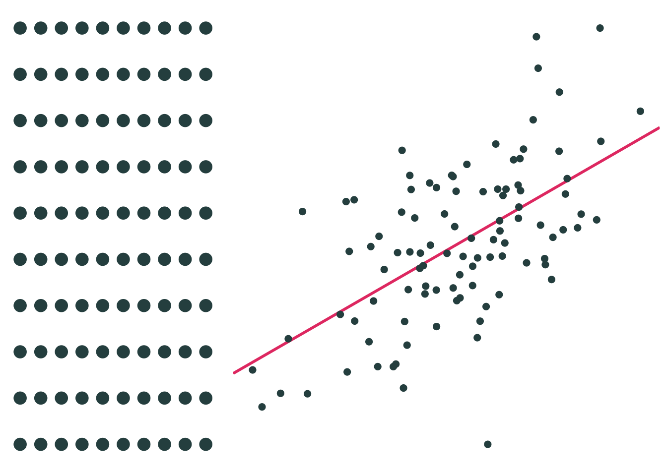

Sample 1: 30 random individuals

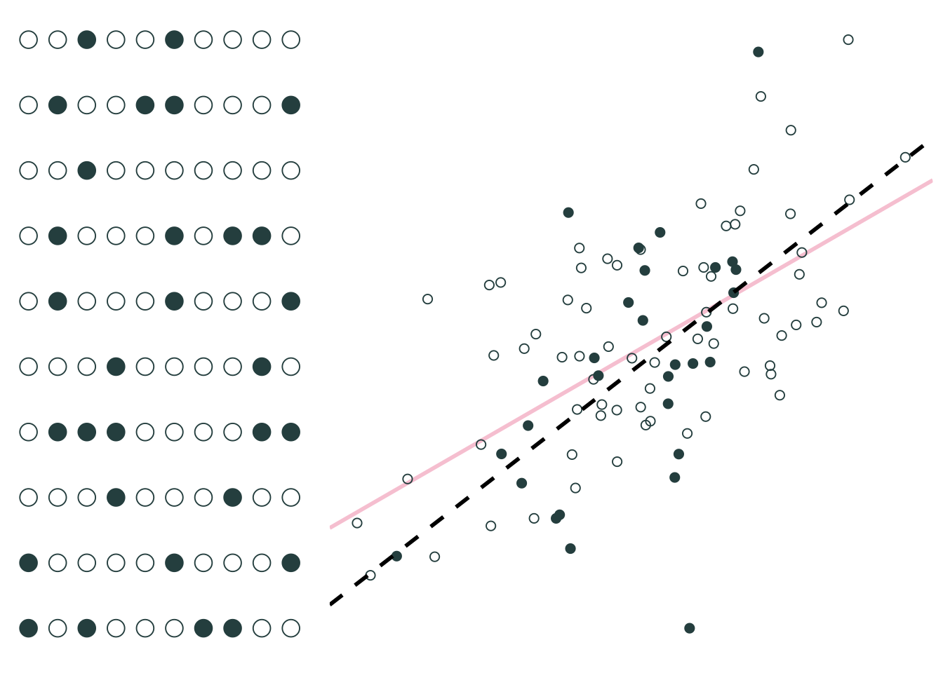
Sample 2: 30 random individuals

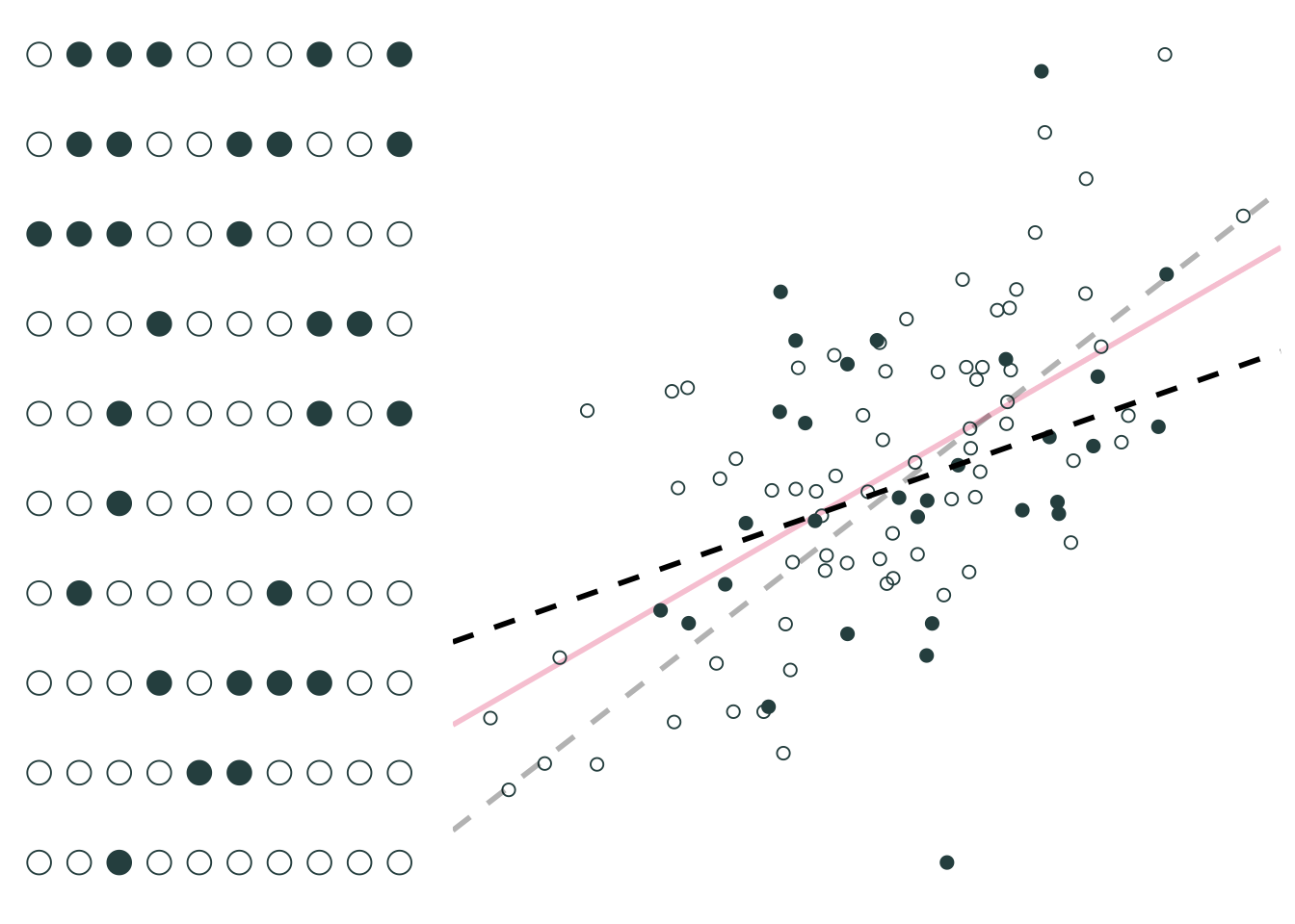
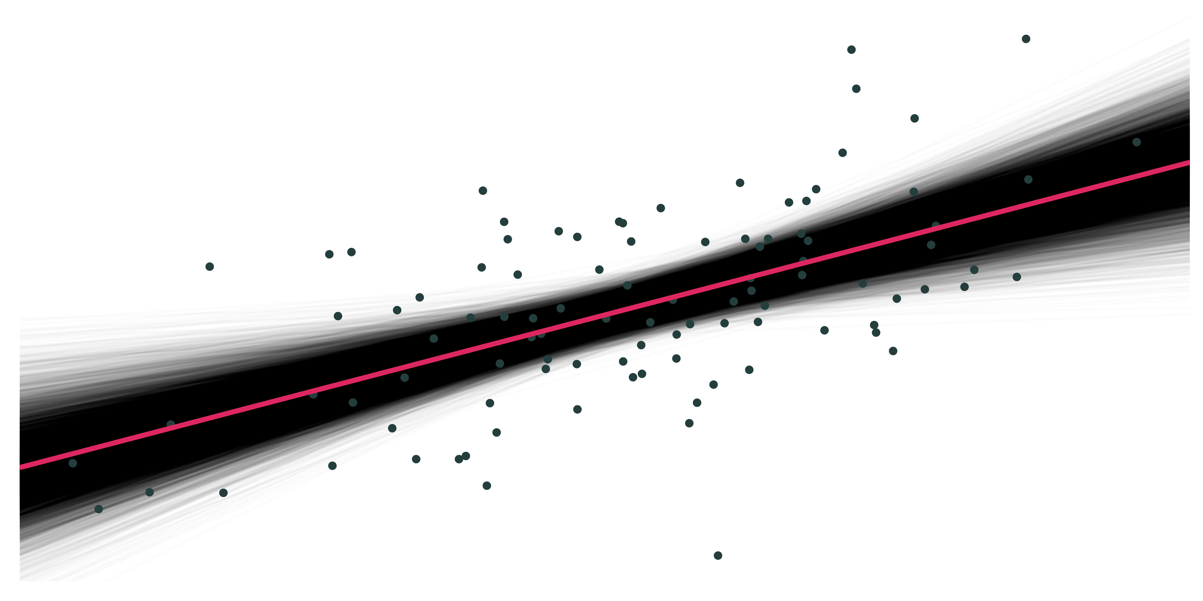
Imagine repeating this 1,000 times, producing a regression equation with each iteration.

What do you notice?

On average, our regression lines match the population line very nicely.
However, individual lines (samples) can really miss the mark.
Differences between individual samples and the population lead to uncertainty for the econometrician.

Answer: Uncertainty matters.

${\hat \beta}$ itself is a random variable—dependent upon the random sample. When we take a sample and run a regression, we don’t know if it’s a “good” sample (${\hat \beta}$ is close to $\beta$) or a “bad sample” (our sample differs greatly from the population).

Keeping track of this and other sources of uncertainty will be a key concept moving forward.

Estimating standard errors for our estimates
Testing hypotheses
Correcting for heteroskedasticity and autocorrelation

But first, let’s remind ourselves of how we get these (uncertain) regression estimates.

Linear regression

The estimator

We can estimate a regression line in R (lm(y ~ x, my_data)) or Stata (reg y x). But where do these estimates come from?

What do we mean by “best-fit line through out data” in describing ${y}_i = {}_0 + {}_1 x_i $?

Being the “best”

Question: What do we mean by best-fit line?

Answers:

In general, best-fit line means the line that minimizes the sum of squared errors (SSE):

\[ \text{SSE} = \sum_{i = 1}^{n} e_i^2 \]

where

\[ e_i = y_i - {\hat y}_i \]

Ordinary least squares (OLS) minimizes the sum of the squared errors.
Based upon a set of (mostly palatable) assumptions, OLS
Is unbiased (and consistent)
Is the best linear unbiased estimator (BLUE… minimum variance.)

OLS vs. other lines/estimators

Let’s consider the dataset we previously generated. For any line (i.e., ${\hat y} = {\hat \beta}_0 + {\hat \beta}_1 x$) that we draw, we can calculate the errors: $e_i = y_i - {\hat y}_i$

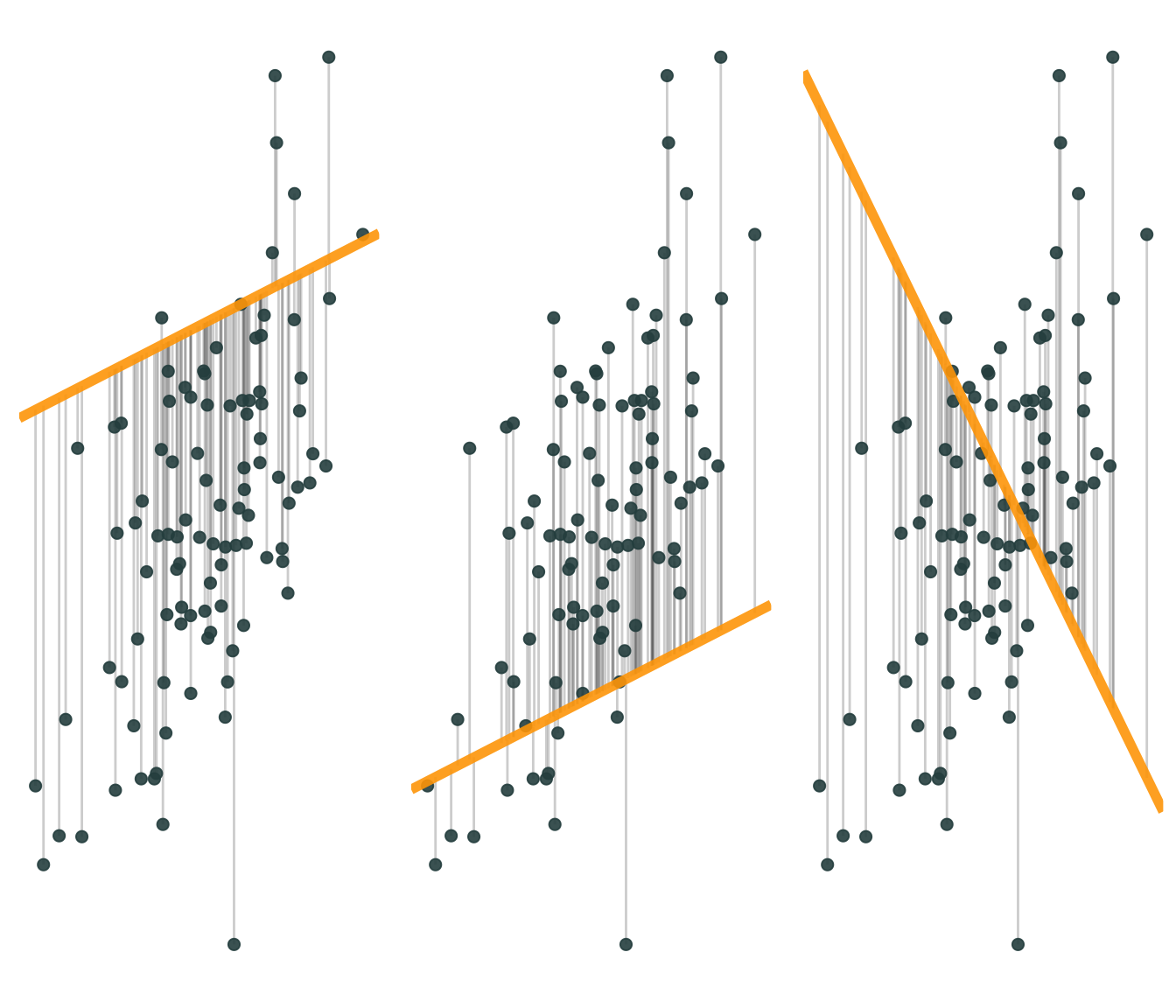
Because SSE squares the errors (i.e., $\sum e_i^2$), big errors are penalized more than small ones.

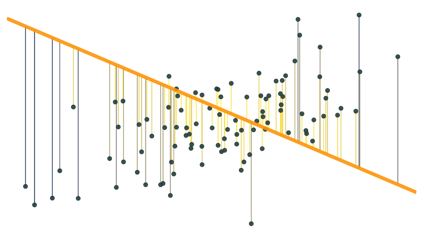
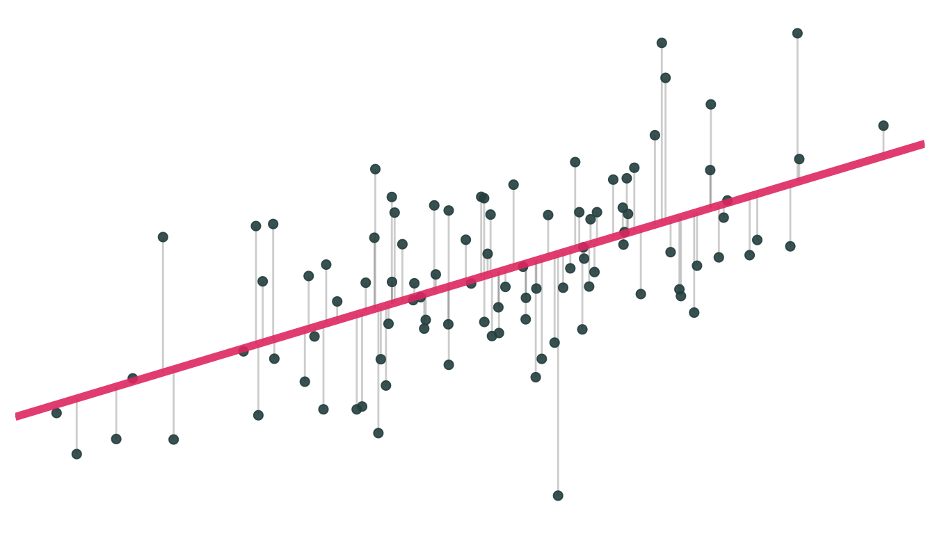
The OLS estimate is the combination of ${\hat \beta}_0$ and ${\hat \beta}_1$ that minimize SSE.

OLS formally

In simple linear regression, the OLS estimator comes from choosing the ${\hat \beta}_0$ and ${\hat \beta}_1$ that minimize the sum of squared errors (SSE), i.e.,

\[ \min_{{\hat \beta}_0,\, {\hat \beta}_1} \text{SSE} \]

But we already know

\[ \text{SSE} = \sum_i e_i^2 \]

Now we use the definitions of $e_i$ and ${\hat y}$ (plus and some algebra)

\[ \begin{aligned} e_i^2 &= \left( y_i - {\hat y}_i \right)^2 = \left( y_i - {\hat \beta}_0 - {\hat \beta}_1 x_i \right)^2 \\ &= y_i^2 - 2 y_i {\hat \beta}_0 - 2 y_i{\hat \beta}_1 x_i + {\hat \beta}_0^2 + 2 {\hat \beta}_0 {\hat \beta}_1 x_i + {\hat \beta}_1^2 x_i^2 \end{aligned} \]

Recall: Minimizing a multivariate function requires (1) first derivatives equal zero (the first-order conditions) and (2) second-order conditions on concavity.

We’re getting close. We need to minimize SSE, and we’ve just shown how SSE relates to our sample (our data, i.e., $x$ and $y$) and our estimates (i.e., ${\hat \beta}_0$ and ${\hat \beta}_1$).

\[ \text{SSE} = \sum_i e_i^2 = \sum_i \left( y_i^2 - 2 y_i {\hat \beta}_0 - 2 y_i {\hat \beta}_1 x_i + {\hat \beta}_0^2 + 2 {\hat \beta}_0 {\hat \beta}_1 x_i + {\hat \beta}_1^2 x_i^2 \right) \]

For the first-order conditions of minimization, we now take the first derivatives (don’t forget to check soc) of SSE with respect to ${\hat \beta}_0$ and ${\hat \beta}_1$.

\[ \begin{aligned} \dfrac{\partial \text{SSE}}{\partial {\hat \beta}_0} &= \sum_i \left( 2 {\hat \beta}_0 + 2 {\hat \beta}_1 x_i - 2 y_i \right) = 2n {\hat \beta}_0 + 2 {\hat \beta}_1 \sum_i x_i - 2 \sum_i y_i \\ &= 2n {\hat \beta}_0 + 2n {\hat \beta}_1 \bar{x} - 2n \bar{y} \end{aligned} \]

where $\bar{x} = \frac{\sum x_i}{n}$ and $\bar{y} = \frac{\sum y_i}{n}$ give the sample means of $x$ and $y$ (sample size $n$).

The first-order conditions state that the derivatives are equal to zero, so:

\[ \dfrac{\partial \text{SSE}}{\partial {\hat \beta}_0} = 2n {\hat \beta}_0 + 2n {\hat \beta}_1 \bar{x} - 2n \bar{y} = 0 \]

which implies

\[ {\hat \beta}_0 = \bar{y} - {\hat \beta}_1 \bar{x} \]

Now for ${\hat \beta}_1$.

Take the derivative of SSE with respect to ${\hat \beta}_1$

\[ \begin{aligned} \dfrac{\partial \text{SSE}}{\partial {\hat \beta}_1} &= \sum_i \left( 2 {\hat \beta}_0 x_i + 2 {\hat \beta}_1 x_i^2 - 2 y_i x_i \right) = 2 {\hat \beta}_0 \sum_i x_i + 2 {\hat \beta}_1 \sum_i x_i^2 - 2 \sum_i y_i x_i \\ &= 2n {\hat \beta}_0 \bar{x} + 2 {\hat \beta}_1 \sum_i x_i^2 - 2 \sum_i y_i x_i \end{aligned} \]

set it equal to zero (first-order conditions, again)

\[ \dfrac{\partial \text{SSE}}{\partial {\hat \beta}_1} = 2n {\hat \beta}_0 \bar{x} + 2 {\hat \beta}_1 \sum_i x_i^2 - 2 \sum_i y_i x_i = 0 \]

and substitute in our relationship for ${\hat \beta}_0$, i.e., ${\hat \beta}_0 = \bar{y} - {\hat \beta}_1 \bar{x}$. Thus,

\[ 2n \left(\bar{y} - {\hat \beta}_1 \bar{x}\right) \bar{x} + 2 {\hat \beta}_1 \sum_i x_i^2 - 2 \sum_i y_i x_i = 0 \]

Multiplying out…

\[ 2n \bar{y}\,\bar{x} - 2n {\hat \beta}_1 \bar{x}^2 + 2 {\hat \beta}_1 \sum_i x_i^2 - 2 \sum_i y_i x_i = 0 \]

\[ \implies 2 {\hat \beta}_1 \left( \sum_i x_i^2 - n \bar{x}^2 \right) = 2 \sum_i y_i x_i - 2n \bar{y}\,\bar{x} \]

\[ \implies {\hat \beta}_1 = \dfrac{\sum_i y_i x_i - 2n \bar{y}\,\bar{x}}{\sum_i x_i^2 - n \bar{x}^2} = \dfrac{\sum_i (x_i - \bar{x})(y_i - \bar{y})}{\sum_i (x_i - \bar{x})^2} \]

With that… we have OLS estimators for the slope,

\[ {\hat \beta}_1 = \dfrac{\sum_i (x_i - \bar{x})(y_i - \bar{y})}{\sum_i (x_i - \bar{x})^2} ~,\]

and intercept,

\[ {\hat \beta}_0 = \bar{y} - {\hat \beta}_1 \bar{x} ~.\]

OLS properties and assumptions

What properties might we care about for an estimator?

Refresher: Density functions

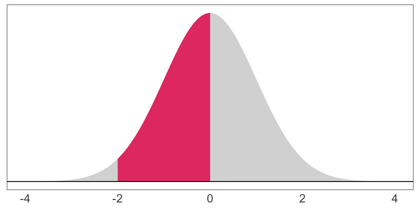
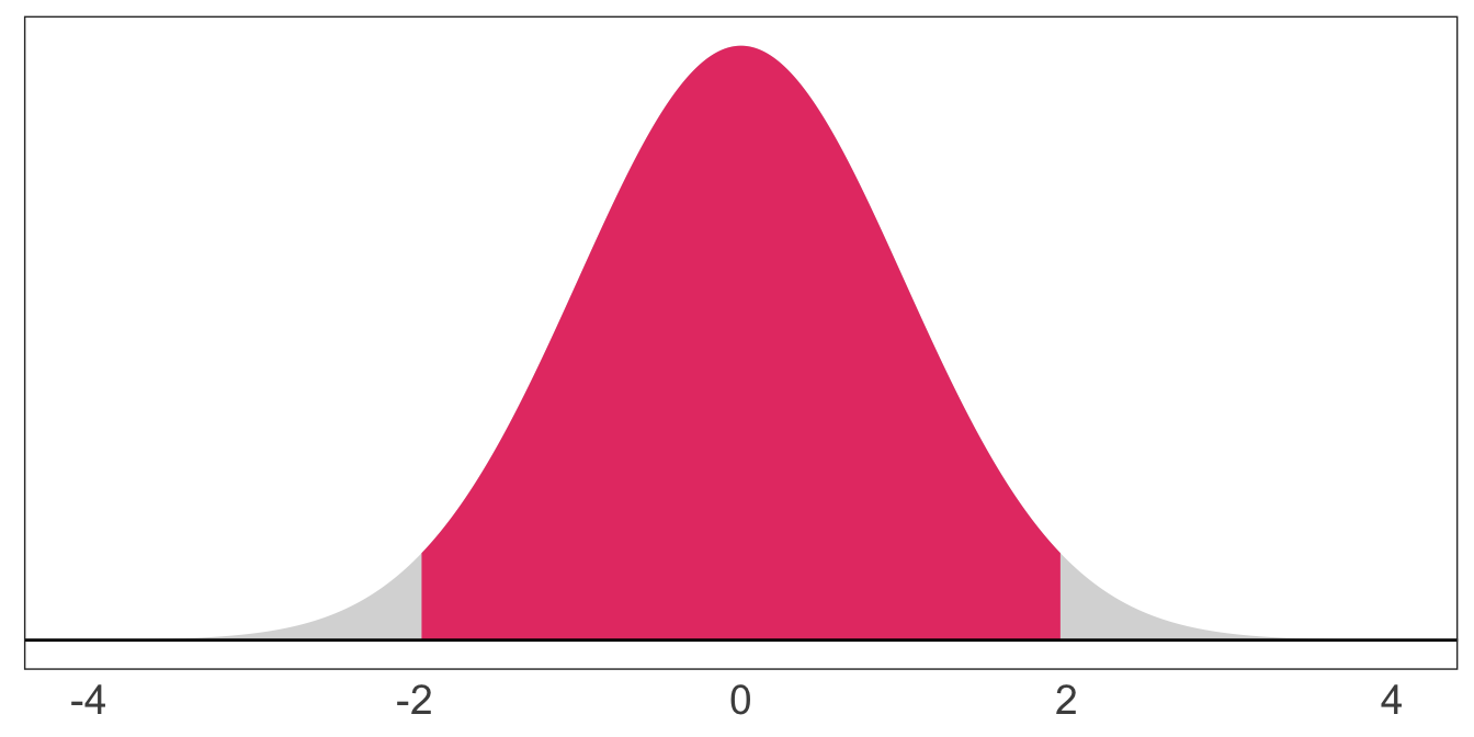
Recall that we use probability density functions (PDFs) to describe the probability a continuous random variable takes on a range of values. (The total area = 1.)

These PDFs characterize probability distributions, and the most common/famous/popular distributions get names (e.g., normal, t, Gamma).

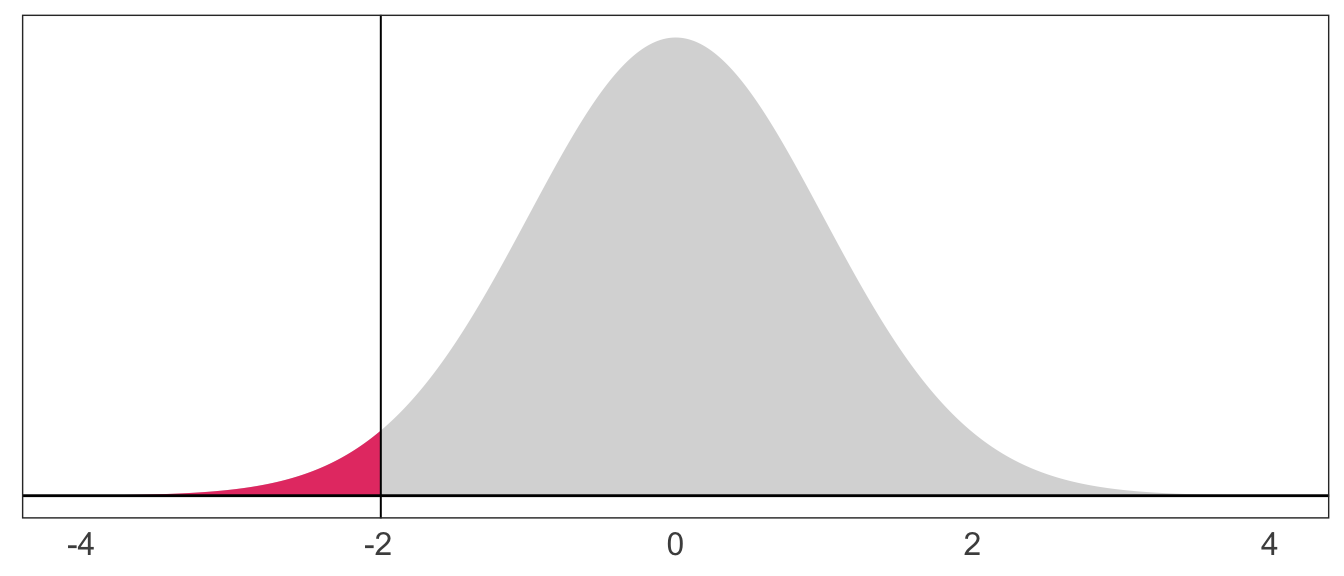
The probability a standard normal random variable takes on a value between -2 and 0: $\mathop{\text{P}}\left(-2 \leq X \leq 0\right) = 0.48$

The probability a standard normal random variable takes on a value between -1.96 and 1.96: $\mathop{\text{P}}\left(-1.96 \leq X \leq 1.96\right) = 0.95$

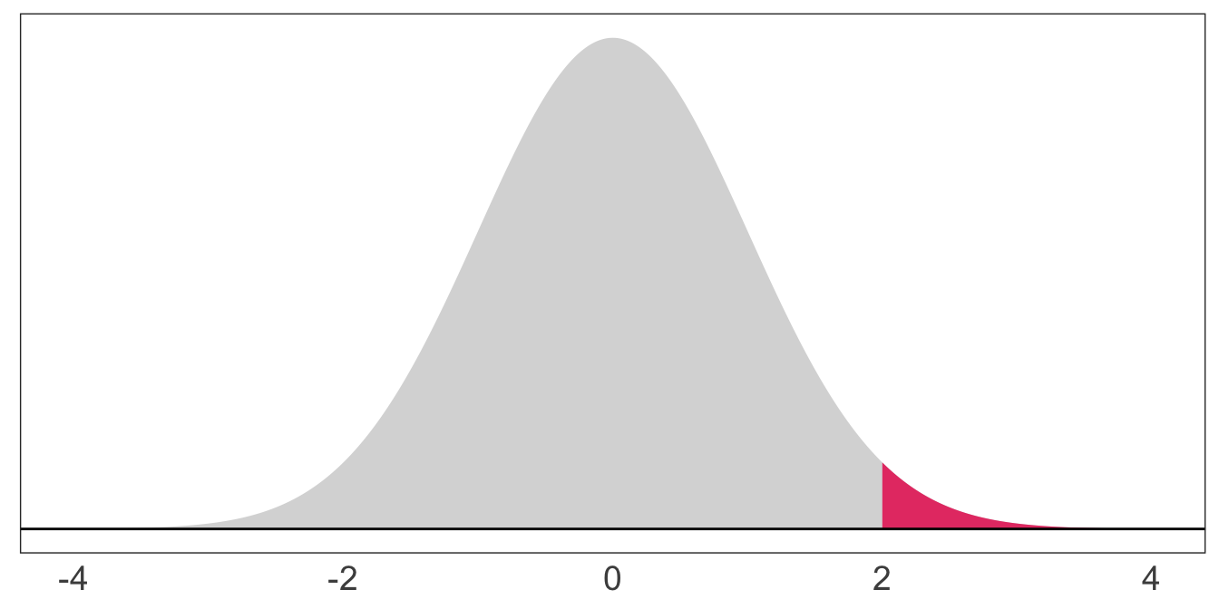
The probability a standard normal random variable takes on a value beyond 2: $\mathop{\text{P}}\left(X > 2\right) = 0.023$

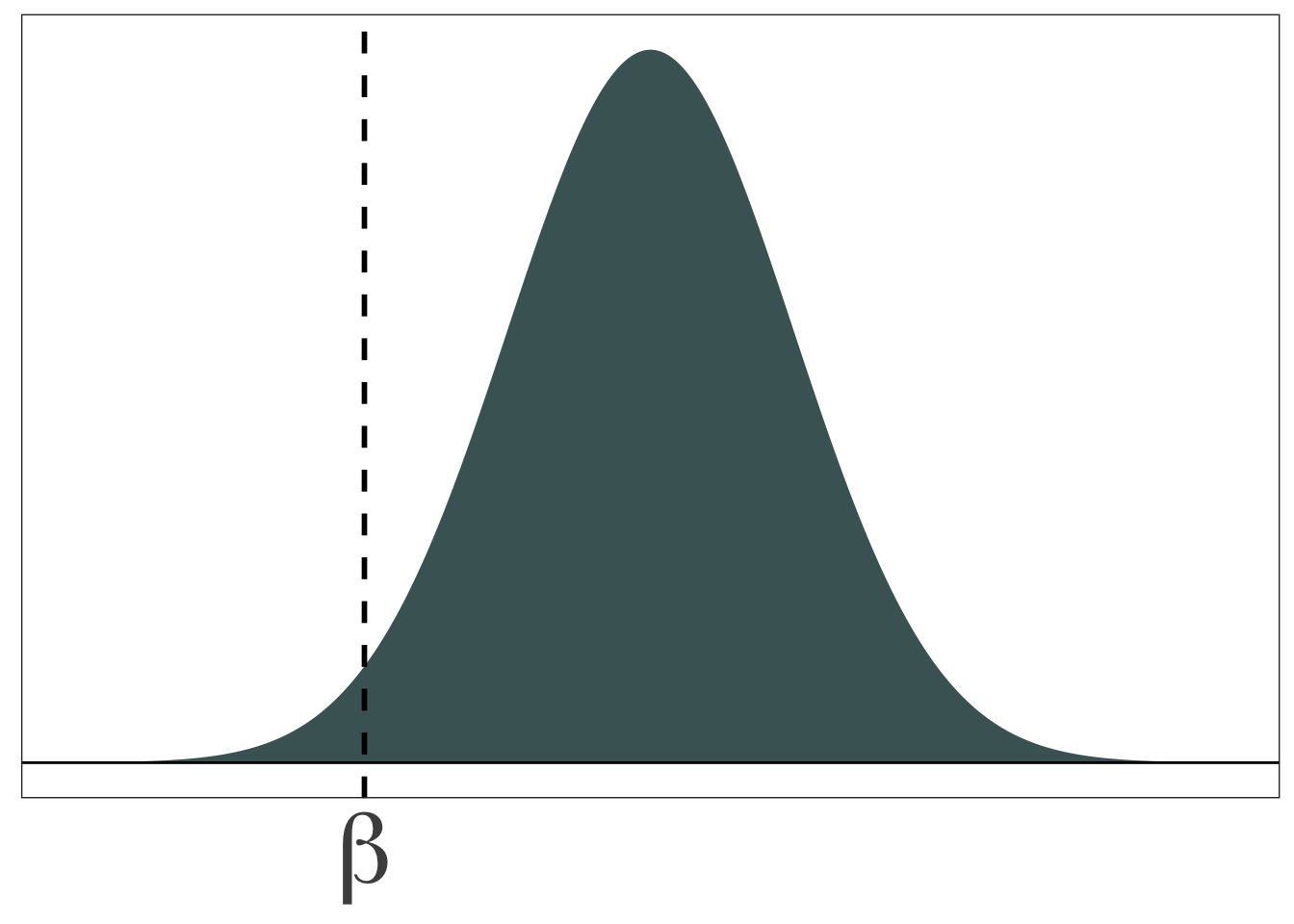
Imagine we are trying to estimate an unknown parameter $\beta$, and we know the distributions of three competing estimators. Which one would we want? How would we decide?

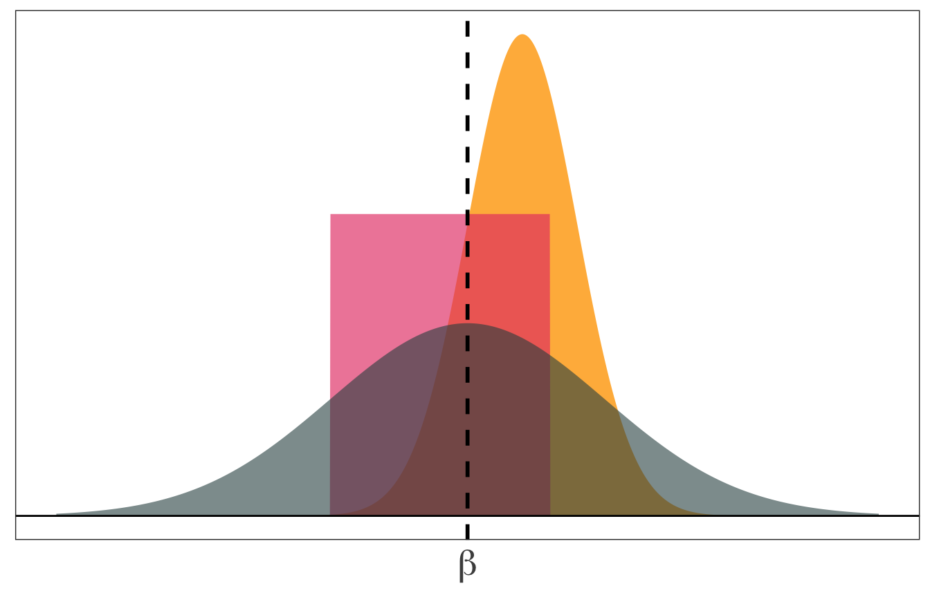
So, what properties might we care about for an estimator?

Answer 1: Bias

On average (after many samples), does the estimator tend toward the correct value?

More formally: Does the mean of estimator’s distribution equal the parameter it estimates?

\[ \mathop{\text{Bias}}_\beta \left( {\hat \beta} \right) = \mathop{\boldsymbol{E}}\left[ {\hat \beta} \right] - \beta \]

Unbiased estimator: $\mathop{\boldsymbol{E}}\left[ {\hat \beta} \right] = \beta$

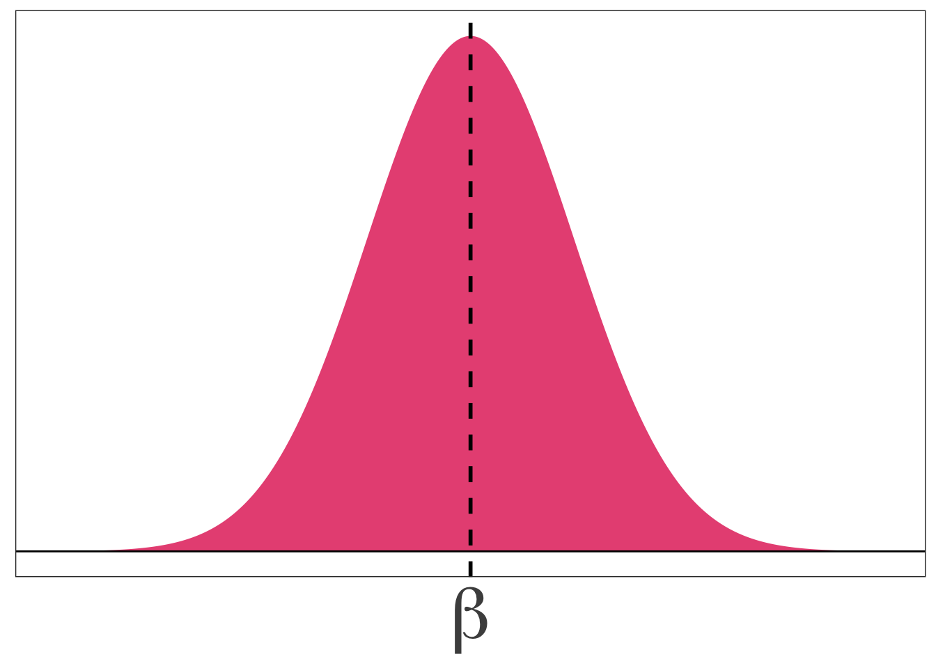
Biased estimator: $\mathop{\boldsymbol{E}}\left[ {\hat \beta} \right] \neq \beta$

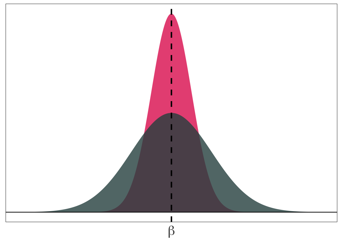
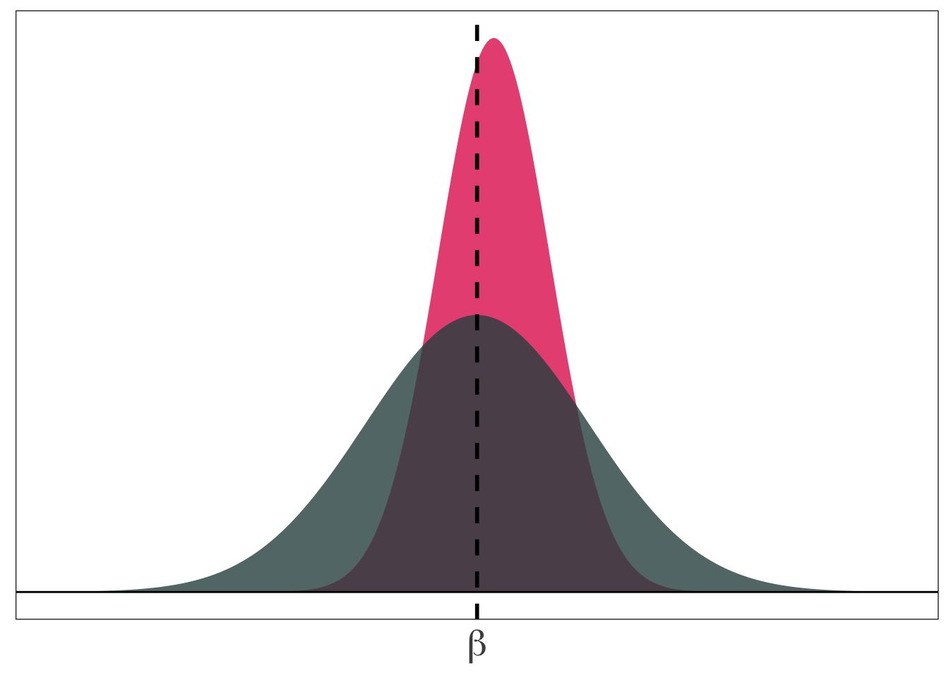
Answer 2: Variance

The central tendencies (means) of competing distributions are not the only things that matter. We also care about the variance of an estimator.

\[ \mathop{\text{Var}} \left( {\hat \beta} \right) = \mathop{\boldsymbol{E}}\left[ \left( {\hat \beta} - \mathop{\boldsymbol{E}}\left[ {\hat \beta} \right] \right)^2 \right] \]

Lower variance estimators mean we get estimates closer to the mean in each sample.

The bias-variance tradeoff

Should we be willing to take a bit of bias to reduce the variance?

In econometrics, we generally stick with unbiased (or consistent) estimators. But other disciplines (especially computer science) think a bit more about this trade off.

OLS Properties

As you might have guessed by now,

OLS is unbiased
OLS has the minimum variance of all unbiased linear estimators

OLS Assumptions

These (very nice) properties depend upon a set of assumptions.

The population relationship is linear in parameters with an additive disturbance.
Our $X$ variable is exogenous, i.e., $\mathop{\boldsymbol{E}}\left[ u | X \right] = 0$.
The $X$ variable has variation. And if there are multiple explanatory variables, they are not perfectly collinear.
The population disturbances $u_i$ are independently and identically distributed as normal random variables with mean zero $\left( \mathop{\boldsymbol{E}}\left[ u \right] = 0 \right)$ and variance $\sigma^2$ (i.e., $\mathop{\boldsymbol{E}}\left[ u^2 \right] = \sigma^2$). Independently distributed and mean zero jointly imply $\mathop{\boldsymbol{E}}\left[ u_i u_j \right] = 0$ for any $i\neq j$.

Assumptions (1), (2), and (3) make OLS unbiased
Assumption (4) gives us an unbiased estimator for the variance of our OLS estimator

Of course, there are many ways that real life may violate these assumptions. For instance:

Non-linear relationships in our parameters/disturbances (or miss-specification)
Disturbances that are not identically distributed and/or not independent
Violations of exogeneity (especially omitted-variable bias)

Uncertainty and inference

Up to this point, we know OLS has some nice properties, and we know how to estimate an intercept and slope coefficient via OLS.

Our current workflow:

Get data (points with $x$ and $y$ values)
Regress $y$ on $x$
Plot the OLS line (i.e., $\hat{y} = {\hat \beta}_0 + {\hat \beta}_1$)
Done?

But how do we actually learn something from this exercise?

Based upon our value of ${\hat \beta}_1$, can we rule out previously hypothesized values?
How confident should we be in the precision of our estimates?
How well does our model explain the variation we observe in $y$?

We need to be able to deal with uncertainty. Enter: Inference.

Learning from our errors

As our previous simulation pointed out, our problem with uncertainty is that we don’t know whether our sample estimate is close or far from the unknown population parameter. (Except when we run the simulation ourselves—which is why we like simulations.)

However, all is not lost. We can use the errors $\left(e_i = y_i - \hat{y}_i\right)$ to get a sense of how well our model explains the observed variation in $y$.

When our model appears to be doing a “nice” job, we might be a little more confident in using it to learn about the relationship between $y$ and $x$.

Now we just need to formalize what a “nice job” actually means.

First off, we will estimate the variance of $u_i$ (recall: $\mathop{\text{Var}} \left( u_i \right) = \sigma^2$) using our squared errors, i.e.,

\[ s^2 = \dfrac{\sum_i e_i^2}{n - k} \]

where $k$ gives the number of slope terms and intercepts that we estimate (e.g., $\beta_0$ and $\beta_1$ would give $k=2$).

$s^2$ is an unbiased estimator of $\sigma^2$.

You then showed that the variance of ${\hat \beta}_1$ (for simple linear regression) is

\[ \mathop{\text{Var}} \left( {\hat \beta}_1 \right) = \dfrac{s^2}{\sum_i \left( x_i - \bar{x} \right)^2} \]

which shows that the variance of our slope estimator

increases as our disturbances become noisier
decreases as the variance of $x$ increases

More common: The standard error of ${\hat \beta}_1$

\[ \mathop{\hat{\text{SE}}} \left( {\hat \beta}_1 \right) = \sqrt{\dfrac{s^2}{\sum_i \left( x_i - \bar{x} \right)^2}} \]

Recall: The standard error of an estimator is the standard deviation of the estimator’s distribution.

Standard error output is standard in .mono[R]’s lm:

tidy(lm(y ~ x, pop_df))

## # A tibble: 2 x 5
##   term        estimate std.error statistic  p.value
##   <chr>          <dbl>     <dbl>     <dbl>    <dbl>
## 1 (Intercept)    2.53     0.422       6.00 3.38e- 8
## 2 x              0.567    0.0793      7.15 1.59e-10

We use the standard error of ${\hat \beta}_1$, along with ${\hat \beta}_1$ itself, to learn about the parameter $\beta_1$.

After deriving the distribution of ${\hat \beta}_1$ – it’s normal with the mean and variance we’ve derived/discussed above – we have two (related) options for formal statistical inference (learning) about our unknown parameter $\beta_1$:

Confidence intervals: Use the estimate and its standard error to create an interval that, when repeated, will generally contain the true parameter. (For example, similarly constructed 95% confidence intervals will contain the true parameter 95% of the time.)
Hypothesis tests: Determine whether there is statistically significant evidence to reject a hypothesized value or range of values.

Confidence intervals

Under our assumptions, we can construct $(1-\alpha)$-level confidence intervals for $\beta_1$ as

\[ {\hat \beta}\_1 \pm t\_{\alpha/2,\text{df}} \, \mathop{\hat{\text{SE}}} \left( {\hat \beta}\_1 \right) \]

$t_{\alpha/2,\text{df}}$ denotes the $\alpha/2$ quantile of a $t$ distribution with $n-k$ degrees of freedom.

For example, 100 obs., two coefficients (i.e., ${\hat \beta}_0$ and ${\hat \beta}_1 \implies k = 2$), and $\alpha = 0.05$ (for a 95% confidence interval) gives us $t_{0.025,\,98} = -1.98$

Example:

lm(y ~ x, data = pop_df) %>% tidy()

## # A tibble: 2 x 5
##   term        estimate std.error statistic  p.value
##   <chr>          <dbl>     <dbl>     <dbl>    <dbl>
## 1 (Intercept)    2.53     0.422       6.00 3.38e- 8
## 2 x              0.567    0.0793      7.15 1.59e-10

Our 95% confidence interval is thus

\[ 0.567 \pm 1.98 \times 0.0793 = \left[ 0.410,\, 0.724 \right] \]

So we have a confidence interval for $\beta_1$, i.e., $\left[ 0.410,\, 0.724 \right]$.

What does it mean?

Informally: The confidence interval gives us a region (interval) in which we can place some trust (confidence) for containing the parameter.

More formally: If repeatedly sample from our population and construct confidence intervals for each of these samples, $(1-\alpha)$ percent of our intervals (e.g., 95%) will contain the population parameter somewhere in the interval.

Now back to our simulation…

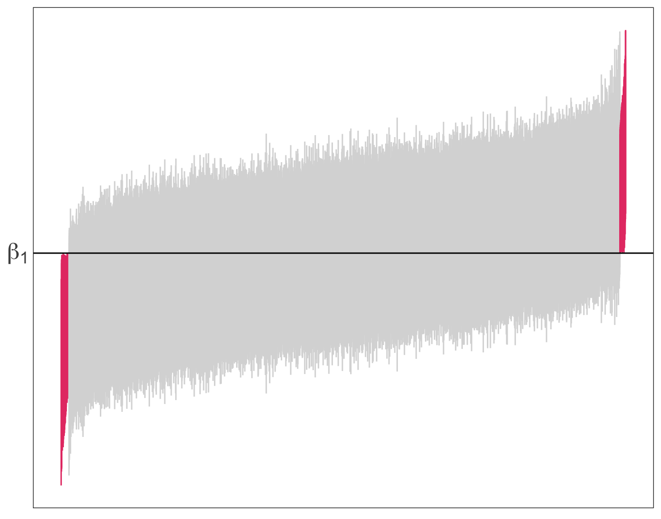
We drew 10,000 samples (each of size $n = 30$) from our population and estimated our regression model for each of these simulations:

\[ y_i = {\hat \beta}_0 + {\hat \beta}_1 x_i + e_i \]

(repeated 10,000 times)

Now, let’s estimate 95% confidence intervals for each of these intervals…

From our previous simulation: 97.6% of 95% confidences intervals contain the true parameter value of $\beta_1$.

Hypothesis testing

In many applications, we want to know more than a point estimate or a range of values. We want to know what our statistical evidence says about existing theories.

We want to test hypotheses posed by officials, politicians, economists, scientists, friends, weird neighbors, etc.

Examples

Does increasing police presence reduce crime?
Does building a giant wall reduce crime?
Does shutting down a government adversely affect the economy?
Does legalizing cannabis reduce drunk driving and/or reduce opiod use?
Do more stringent air quality standards increase birthweights and/or reduce jobs?

Hypothesis testing relies upon very similar results and intuition as confidence intervals.

While uncertainty certainly exists, we can build statistical tests that generally get the answers right (rejecting or failing to reject a posited hypothesis).

OLS $t$ test

Imagine a (null) hypothesis which states that $\beta_1$ is equal to some value $c$, i.e., $H_o:\: \beta_1 = c$

From OLS’s properties, we can show that the test statistic

\[ t_\text{stat} = \dfrac{{\hat \beta}_1 - c}{\mathop{\hat{\text{SE}}} \left( {\hat \beta}_1 \right)} \]

follows the $t$ distribution with $n-k$ degrees of freedom.

For an $\alpha$-level, two-sided test, we reject the null hypothesis (and conclude with the alternative hypothesis) when

\[\left|t\_\text{stat}\right| > \left|t\_{1-\alpha/2,\,df}\right|,\]

meaning that our test statistic is more extreme than the critical value.

Alternatively, we can calculate the p-value that accompanies our test statistic, which effectively gives us the probability of seeing our test statistic or a more extreme test statistic if the null hypothesis were true.

Very small p-values (generally < 0.05) mean that it would be unlikely to see our results if the null hypothesis were really true—we tend to reject the null for p-values below 0.05.

Example

Standard .mono[R] and .mono[Stata] output tends to test hypotheses against the value zero.

lm(y ~ x, data = pop_df) %>% tidy()

## # A tibble: 2 x 5
##   term        estimate std.error statistic  p.value
##   <chr>          <dbl>     <dbl>     <dbl>    <dbl>
## 1 (Intercept)    2.53     0.422       6.00 3.38e- 8
## 2 x              0.567    0.0793      7.15 1.59e-10

$H_o:\: \beta_1 = 0$ and $H_a:\: \beta_1 \neq 0$

$t_\text{stat} = 7.15$ and $t_\text{0.975, 28} = 2.05$

$\text{p-value} < 0.05$

Reject $H_o$

Back to our simulation! Let’s see what our $t$ statistic is actually doing.

In this situation, we can actually know (and enforce) the null hypothesis, since we generated the data.

For each of the 10,000 samples, we will calculate the $t$ statistic, and then we can see how many $t$ statistics exceed our critical value (2.05, as above).

The answer should be approximately 5 percent—our $\alpha$ level.

In our simulation, 2.4 percent of our $t$ statistics reject the null hypothesis.

The distribution of our $t$ statistics (shading the rejection regions).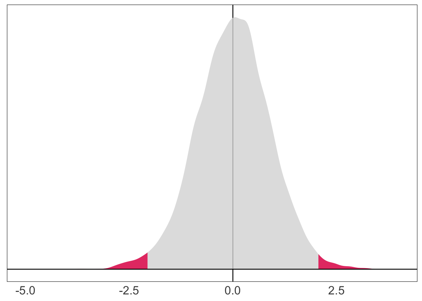

Correspondingly, 2.4 percent of our p-values reject the null hypothesis.

The distribution of our p-values (shading the p-values below 0.05).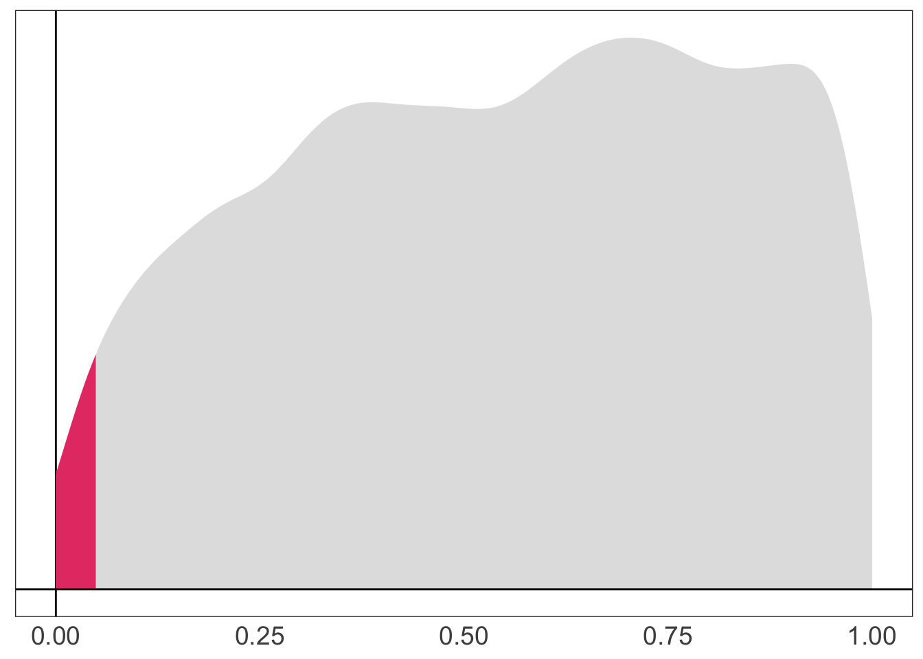

F tests

Example

Economists love to say “Money is fungible.”

Imagine that we might want to test whether money received as income actually has the same effect on consumption as money received from tax rebates/returns.

\[ \text{Consumption}_i = \beta_0 + \beta_1 \text{Income}_{i} + \beta_2 \text{Rebate}_i + u_i \]

We can write our null hypothesis as

\[ H_o:\: \beta_1 = \beta_2 \iff H_o :\: \beta_1 - \beta_2 = 0 \]

Imposing this null hypothesis gives us the restricted model

\[ \text{Consumption}_i = \beta_0 + \beta_1 \text{Income}_{i} + \beta_1 \text{Rebate}_i + u_i \] \[ \text{Consumption}_i = \beta_0 + \beta_1 \left( \text{Income}_{i} + \text{Rebate}_i \right) + u\_i \]

Example

To this the null hypothesis $H_o :\: \beta_1 = \beta_2$ against $H_a :\: \beta_1 \neq \beta_2$, we use the $F$ statistic

\[ F\_{q,\,n-k} = \dfrac{\left(\text{SSE}\_r - \text{SSE}\_u\right)/q}{\text{SSE}\_u/(n-k-1)} \]

which (as its name suggests) follows the $F$ distribution with $q$ numerator degrees of freedom and $n-k$ denominator degrees of freedom.

The term $\text{SSE}_r$ is the sum of squared errors (SSE) from our restricted model \[ \text{Consumption}_i = \beta_0 + \beta_1 \left( \text{Income}_{i} + \text{Rebate}_i \right) + u\_i \]

and $\text{SSE}_u$ is the sum of squared errors (SSE) from our unrestricted model \[ \text{Consumption}_i = \beta_0 + \beta_1 \text{Income}_{i} + \beta_2 \text{Rebate}_i + u_i \]