Chapter 6 Matching

Matching is a non-parametric or semi-parametric analogue to regression that is used for the evaluation of binary treatments. It uses non-parametric regression methods to construct counterfactuals under an assumption of selection on observables. (It’s time has past… though still lives on in the consulting world.)

Since Rosenbaum and Rubin (Biometrika, 1983), the propensity score matching (PSM) approach has gained increasing popularity among researchers in a wide range of disciplines: bio-medical research, epidemiology, public health, economics, sociology, and psychology. Heckman’s contribution—especially his difference-in-differences method—produced a major change in standard approaches to program evaluation (Heckman, Ichimura, and Todd (REStud 1997)).

In matching, we brute-force the construction of appropriate counterfactuals
- Can use non-parametric or semi-parametric regression methods to aid with this
But, like OLS, we must assume that selection is on observables
- If you can see all the $X$’s that lead to treatment, and are willing to assume that there are no others $\rightarrow$ causality!
Propensity score matching (PSM) has gained increasing popularity among researchers in a wide range of disciplines: bio-medical research, epidemiology, public health, economics, sociology, and psychology.
- Similar to assuming that $Cov(u_i, y_i)=0$ in OLS

In the absence of ex ante randomization, a potential substitute would be to match treated entities with untreated entities that are “identical” or near-identical on observable characteristics.

The average outcome for the matched group (who weren’t treated) operates as a stand in for the counter-factual outcomes for the treated group in the absence of treatment.
Assumes that there is not some unobservable characteristic that differs across these groups and significantly affects both treatment propensity and the outcome variable.

Estimates of the treatment effect are then the average difference between the outcome levels of treated entities and the outcome levels of their matched controls.

Example 1: Exact matching

Suppose you were interested in the effect of a job-training programme on earnings.

What is your prior… i.e., your expectation about the effect of training on earnings?

Q: If trainees were younger… would you expect a comparison of trainees and non-trainees to be an unbiased estimate of the causal effect of training?

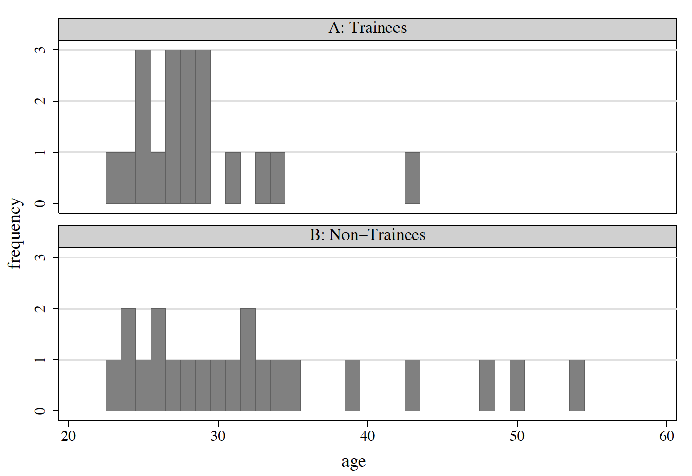
Figure 6.1: Age Distributions: Before Matching

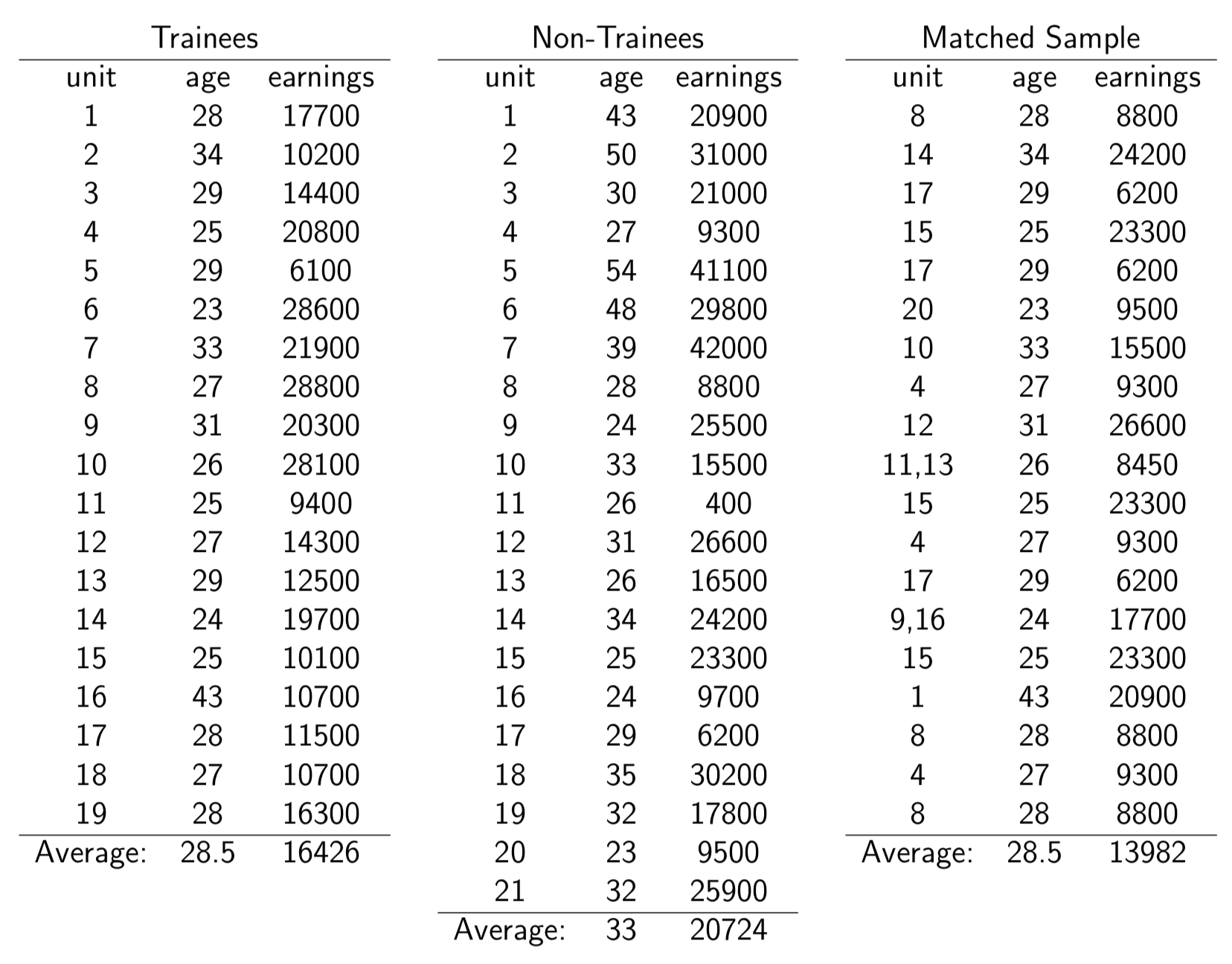
Figure 6.2: Comparing matched and matched samples

Suppose we define training-effect estimates as the difference in average earnings between trainees and non-trainees

Before matching: 16,426 - 20,724 = -4,298
After matching: 16,426 -13,982 = 2,444

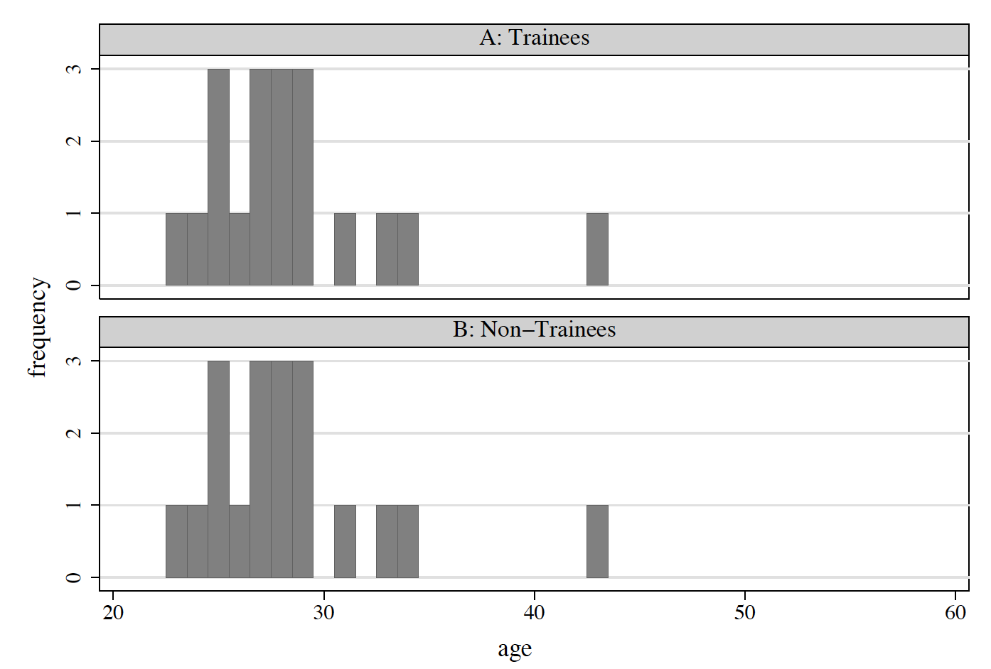
Figure 6.3: Age Distributions: After Matching

More generally…

Consider a non-experimental context in which there is no true randomization of assignment to “treatment” and “control” groups—entities sort themselves into these two groups in some non-experimental fashion. (Recall that if we had truly randomized treatments, we could confidently look at a difference in mean outcomes across the two groups and attribute this difference to treatment.)

A potential substitute would be to match data for treated entities with data for some untreated entity that is identical or near-identical on observable characteristics.
The average outcome for the untreated matched group stands in for the counter-factual mean outcome for the treated group in the absence of treatment—provided there is not some unobservable characteristic that differs across these groups and significantly affects both treatment propensity and the outcome variable.
Estimates of the treatment effect are then given by the average across the treated of the difference between the outcome level for the treated entity and the outcome level (or average outcome level) among the matched controls.

Let $Y_1$ denote the outcome (e.g., earnings) in the “treated” state and let $Y_0$ denote the outcome in the untreated state.

Let $D$ be an indicator variable denoting participation in the program. The observed outcome is then $Y=DY_1+(1-D)Y_0$.

The Average Treatment Effect (ATE): $\Delta^{ATE}= E(Y_1-Y_0)= E(Y_1)-E(Y_0)$
The Treatment on the Treated (TT): $\Delta^{TT} = E(Y_1-Y_0 \mid D=1) = E(Y_1 \mid D=1)-E(Y_0 \mid D=1)$

As before, these parameters answer different policy questions. They also require different assumptions to be made when using matching methods.

The evaluation problem arises again because we can only observe one of $\{Y_1,Y_0\}$ for each person. As in previous environments, we do not observe the untreated outcome for the treated or the treated outcome for the untreated. With this in mind, consider estimating $\Delta^{TT} = E(Y_1 \mid D=1)-E(Y_0 \mid D=1)$, for example.

We can construct $E(Y_1 \mid D=1)$ from data on the treated, but we do not observe $E(Y_0 \mid D=1)$.
If we substitute data on the untreated outcome for the untreated, we have selection bias equal to $E(Y_0 \mid D=1)-E(Y_0 \mid D=0)$. It results from the fact that, in general, people do not select into treatment in a way that is unrelated to the untreated outcome.

Random-assignment experiments solve the evaluation problem by direct construction of the unobserved counterfactual $E(Y_0 \mid D=1)$… forcibly and randomly excluding $D=1$ persons who would otherwise have been treated from the treatment. In contrast, matching solves the evaluation problem by assuming that selection is unrelated to the untreated outcome conditional on some set of observed variables, $X$.

The conditional independence assumption (CIA)

The primary assumption that underlies matching is the conditional independence (CIA). The CIA states that treatment status is random conditional on some set of observed $X$ variables. In notation, the CIA is given by $(Y_0 \perp D) \mid X$ for the treatment on the treated parameter and by $(Y_0 ,Y_1)\perp D \mid X$ for the average treatment effect parameter.

The applied literature sometimes claims that matching is more “like” random assignment than other non-experimental evaluation methods insofar as matching, like random assignment, balances the distributions of both observables and unobservables between the treated and untreated units. Similarly, matching balances the observables between the treated and untreated units. More generally, however, matching is no more “like” random assignment than any other non-experimental evaluation method, as all such methods are “like” random assignment when the assumptions that justify them hold in the data.

(This point is key to much of what we are discussing this term.)

Example 2

Suppose that we are interested in estimating the impact of treatment on the treated: \[ \Delta^{TT}=E(Y_1 -Y_0 \mid D=1)=E(Y_1 \mid D=1)-E(Y_0 \mid D=1).\] Suppose also that $X \in \{M,F\}$, that there are 100 people in each group in the population, and that \[ Pr(D=1 \mid X=M)=0.6 \text{, and, } Pr(D=1 \mid X=F)=0.4 \] \[ E(Y_0 \mid X =M)=20 \text{, and, } E(Y_0 \mid X = F)=10 \] In this example, we have selection on $Y_0$ via selection on $X$. (If $X$ is not observed, we have selection on unobservables. If $X$ is observed, we have selection on observables.)

If $\Delta =Y_1-Y_0 = 5$ (by assumption), the simple mean-difference impact estimator, $E(Y_1)-E(Y_0)$, is easily constructed: \[E(Y_1)=(0.6)(20 + 5) + (0.4)(10 + 5) = 15 + 6 = 21\] \[ E(Y_0)=(1-0.6)(20)+(1-0.4)(10) = 8 + 6 =14\] The simple mean difference impact estimator gives an impact of ${\hat \Delta}=7 \ne 5$.

What does matching do? In matching, we construct a separate impact estimate for each $X$ and then take a weighted average, where the weights are the fractions of each $X$ group in the treated population. Thus, \[ E(Y_1 \mid D=1,X =M)=25\] \[E(Y_1 -Y_0 \mid D=1,X=M)=25-20=5\] Similarly (repeat the steps), \[E(Y_1-Y_0 \mid D=1,X=F)=5.\] Thus,\[E(Y_1-Y_0 \mid D=1) = Pr(X=M \mid D=1) \cdot E(Y_1-Y_0 \mid D=1,X=M) +\] \[Pr(X=F \mid D=1) \cdot E(Y_1-Y_0 \mid D=1,X=F).\]

Substitution yields $E(Y_1 - Y_0 \mid D=1)=(0.6)(5)+(0.4)(5)=5$. (Note that the last step was superfluous here because we assumed homogeneous impact for the two groups, but would be required in general.)

Traditional regression analysis also assumes that selection into treatment is “on the observables,” and can therefore be eliminated by conditioning on those observables.

Given that regression is simpler than matching, why not just run regressions instead? Matching affords three things that standard regression analysis does not:

Matching does not make the linear functional-form assumption that regression does. If the CIA holds, but linearity does not, then matching is consistent (while regression is not).
Matching highlights the support problem in a way that regression does not. Put simply, matching makes it evident whether or not comparable untreated observations are available for each treated observation. As such, it helps one avoid identifying effects solely by projections into regions where there are actually no data points. (If there are several discrete $X$s, each with several values, which may include discretized continuous variables, the number of cells may become large, and many cells will have no untreated observations corresponding to each treated observation. For example, if you have five variable each with three values, you have $3^5 = 243$ cells. This is the matching version of the curse of dimensionality. It is a version of the common-support problem.)
Matching weights the observations differently in calculating the expected counterfactual for each treated observation. In OLS, all of the untreated units play a role in determining the expected counter factual for any given treated unit. In contrast, matching dictates that only untreated units similar in observables to each treated unit have positive weight in determining the expected counter factual.

Types of matching

Exact matching

The simplest version of matching is “exact” matching. This technique matches each treated unit to all possible control units with exactly the same values on all covariates. This forms sub classes such that, within each subclass, all units (treatment and control) have the same covariate values. Exact matching is practical when the vector of covariates includes only discrete variables and the sample contains many observations across each distinct pattern of these variables.

Inexact matching

When the curse of dimensionality strikes, matching estimators that do not require exact matching pose a solution. Inexact-matching procedures reduce the dimensionality of the problem by defining a distance metric on $X$ and then matching using the distance rather than the $X$. For example, you can construct the Mahalanobis distance between each treated observation and each untreated observation and match on that by defining $w(i,j)$ in terms of the distance. Asymptotically, all inexact matching schemes are in some sense equivalent since they all tend toward exact matches as the sample gets larger. However, they can yield very different answers in finite samples.

Consider the problem of estimating the probability that a test point in N-dimensional Euclidean space belongs to a set, where we are given sample points that definitely belong to that set. Our first step would be to find the average or center of mass of the sample points. Intuitively, the closer the point in question is to this center of mass, the more likely it is to belong to the set. However, we also need to know if the set is spread out over a large range or a small range, so that we can decide whether a given distance from the center is noteworthy or not. The simplistic approach is to estimate the standard deviation of the distances of the sample points from the center of mass. If the distance between the test point and the center of mass is less than one standard deviation, then we might conclude that it is highly probable that the test point belongs to the set. The further away it is, the more likely that the test point should not be classified as belonging to the set.

If the covariate vector has a large number of variables, or if some variables are continuous so that perhaps no more than one entity may have the same specific value of such variables, one might map $x$ into a lower dimensional measure (perhaps intervals of each continuous variable, such as deciles, or percentiles in a huge sample… or by processing the $x$ vector through a function to produce a scalar $f(x)$ that facilitates matching.

Propensity score matching

Propensity Score Matching (PSM) is a popular strategy for generating inexact matches. A “propensity score” is simply the conditional probability of treatment participation given $X$, typically denoted $P(X_i)$. It is often calculated from a binary discrete-choice model (e.g., logit) to explain the “treatment” or “non-treatment” status of an individual in the sample as a function of observable attributes. This makes use of an important result:

If selection bias can be eliminated by controlling for the levels of each of the variables in $X$, it is also eliminated by controlling for the propensity score, which is often easier to do.

It is Rosenbaum and Rubin (Biometrika, 1983) that shows that if you can match on $X$ then you can also match on $P(X)=Pr(D=1 \mid X)$…the so-called propensity score.

The intuition is that two groups with the same probability of participation will show up in the treated and untreated samples in equal proportions. Thus, they can be combined for purposes of comparison.

Suppose the following: \[\text{100 Bikers: } E(Y_0)=10, E(Y_1)=20, Pr(D=1)=0.8\] \[\text{100 Hikers: } E(Y_0) =100, E(Y_1)=200, Pr(D=1) = 0.8\] These assumptions imply that there are 20 bikers and 20 hikers in the comparison group, so that \[ E(Y_0 \mid D = 0) = \frac{20}{20+20}(10)+\frac{20}{20+20}(100)=(.5)(10)+(.5)(100)=5+50=55,\] and 80 bikers and 80 hikers in the treated group, so that \[ E(Y_0 \mid D = 1) = \frac{80}{80+80}(10)+\frac{80}{80+80}(100)=(.5)(10)+(.5)(100)=5+50=55.\] Why can you combine these groups? Because the relative proportions will always be the same in the treatment and comparison groups.

You can see this by repeating the previous example with 100 bikers and 1,000 hikers, where there would be 20 bikers and 200 hikers in the comparison group, and 80 bikers and 800 hikers in the treatment group. Again, one would have, \[ E(Y_0 \mid D = 0) = \frac{20}{200+20}(10)+\frac{200}{200+20}(100)=\frac{1}{11}(10)+\frac{1}{11}(100)= 110/11\] \[ E(Y_0 \mid D = 1) = \frac{80}{80+800}(10)+\frac{800}{80+800}(100)=\frac{1}{11}(10)+\frac{1}{11}(100)= 110/11\] Note that the treatment effect for the combined group is a weighted average of the treatment effects of the two groups, with the weights being their proportion in the treated group, if the treatment on the treated parameter is being estimated.

Another way to think of this is that if $Y_0$ is independent of $D$ given $X$, then it should also be independent of $D$ conditional on $P(X)$ (which summarizes the information in $X$ relative to $D$). (Think balance test… we’ll return to that intutition later.)

Estimating the propensity score

Suppose you want to estimate the propensity score non-parametrically. To do so, you would compute the probability of participation separately for cells defined by $X$, and you would be right back to the curse of dimensionality. In fact, the propensity score is almost always estimated using a parametric model such as a logit or a probit.
The primary justification given for this practice is that Monte Carlo evidence and evidence from sensitivity analyses imply that parametric estimation of the propensity score makes very little difference. Note too that the approximation error associated with a parametric model may be less for a binary dependent variable (as in the participation equation) than for a continuous dependent variable (as in the outcome equation in most cases).
- It is important to adopt a flexible specification for the parametric propensity score in practice and to select that specification via balancing tests.

Nearest-neighbour matching

This is the most common form of matching in the statistics literature. For the treatment on the treated parameter, each treated person is matched to the nearest untreated person.

Should you match with replacement? That is, should a given treated observation form the counterfactual for more than one treated observation?

Matching without replacement can yield very poor matches if the number of comparison observations (i.e., those with $D=0$) comparable to the treated observations is small.
Matching without replacement does keep the variance low at the cost of potential bias while matching with replacement keeps bias low at the cost of a larger variance.
Matching without replacement is order dependent, though there are variants, called “optimal matching” in the applied statistics literature, that try to find the best (by some distance criterion) set of matches without replacement. See Hansen (JASA 2004).

Whether or not to match with replacement depends in part on the data (e.g., whether there is a unique close match for each treated observation).

Kernel matching

Kernel matching takes local averages of the comparison group ($D = 0$) observations near each treated observation to construct the counter factual for that observation. \[ w(i,j)=\frac{G_{ij}}{\sum_{k \in \{D_k=0\}}G_{ik}},\] where \[ G_{ik}=G\left( \frac{P(X_i)-P(X_k)}{a_n}\right)\] is a kernel and $a_n$ is a bandwidth parameter that you promise to make smaller as your sample gets larger. The denominator insures that the weights sum to one. Commonly used kernels include the normal kernel, in which $G$ is the normal pdf, the triangle kernel, and the Epanechnikov kernel. (See Cameron and Trivedi, Microeconometrics: Methods and Applications, 2005, Section 9.3, for more.)

You can think about kernel matching as running a weighted regression for each treated observation using the comparison group data where the weights are as above and the regression includes only an intercept term. The coefficient on the intercept is then the estimated counter factual.

Still-other types of matching

Interval matching (or stratification) is very common in the applied statistics literature. It consists of dividing the range of propensity scores into a fixed number of intervals (which need not be of equal length). An interval-specific estimate is obtained by taking the difference between the mean outcomes of the treated and untreated units in each interval. A weighted average of the interval-specific impacts based on the distribution of the treated units among the intervals estimates the treatment on the treated parameter. A weighted average using all of the observations estimates the ATE parameter. (A very nice feature of this estimator is that it avoids the bandwidth selection problem.)
In inverse-probability weighting you can figure out the expected untreated outcome by re-weighting the observed values using the probabilities. In this sense, inverse probability weighting is very similar to undoing stratified sampling except that the probabilities are estimated rather than known.
Radius matching takes the mean of the outcomes for untreated units within a fixed radius of each treated unit as the estimated expected counter factual. The bandwidth problem here takes the form of picking the radius.
Mahalanobis matching involves weighting by covariance matrix of $x$ variables for control group and the difference between the $i^{th}$ treated unit and selected control units.
Local linear matching extends the kernel idea above (of running a weighted regression for each treated observation using the comparison group data where the weights are as above and the regression includes only an intercept term) but includes a linear term in $P(X)$. Local linear matching converges faster at boundary points and can adapt better to different data densities.

Bandwidth selection

The basics

There is a small literature on choosing the bandwidth, which includes rules of thumb based on assumptions about the data generating process, as well as methods for allowing the data to select the bandwidth, such as cross-validation.

There are also schemes for “data dependent bandwidths” in which the bandwidth depends on the density of data nearby. Note that nearest neighbor matching is a form of data dependent bandwidth.

Places to look for discussions of bandwidth selection include Silverman’s book on density estimation and the Pagan and Ullah book on Nonparametric Econometrics.

In practice, ocular selection, combined with some sensitivity analysis and perhaps a rule of thumb or two, is the most common method. However, cross-validation is probably a better choice. We consider it now.

Cross-validation

Cross validation selects bandwidths based on minimizing a mean-squared-error criterion using subsets of the data.

Consider the method of “leave one out” cross-validation (there are other cross validation methods that are similar in spirit but different in details). Let \[ {\hat E}_{-j}(Y_{o,j} \mid P(X_j),bw_k)\] denote the predicted value at $X_j$ obtained from a non-parametric regression of $Y_o$ on $P(X)$ using all of the observations other than observation $j$ and candidate bandwidth $bw_k$.

The estimated mean squared error associated with bandwidth $k$ is given by: \[ {\bar MSE}(bw_k)\sum_{j \in \{D_i=0\}} \frac{1}{n_0}\left[ Y_{0j}-{\hat E}_{-j}(Y_{0,j} \mid P(X_j),bw_k)\right]^2.\] In words, for each untreated unit, you use the candidate bandwidth and the other untreated units to construct an estimated expected value given that unit’s propensity score. Then calculate and square the distance between the actual outcome for that unit and the estimate. Sum the squared errors across observations and take the mean.

Cross validation then selects the bandwidth that minimizes this criterion function.

Choosing a matching method

All matching estimators are consistent (given certain promises about bandwidth choice as the sample size increases), because as the sample gets arbitrarily large, the units being compared get arbitrarily close to one another in terms of their characteristics.

In finite samples, which method one chooses can make a difference and the tradeoffs depend on the data.

If comparison observations are few, single nearest-neighbor matching without replacement is a bad idea.
If comparison observations are many and are evenly distributed, multiple nearest-neighbor matching will make use of the rich comparison group data.
If comparison observations are many but asymmetrically distributed, kernel matching is helpful because it will use the additional data where it exists, but not take bad matches where it does not exist.
If many observations have $P(X)$ near zero or one (the boundaries of the parameter space, as probabilities must be in $[0,1]$ local linear matching is a good idea. Frlich (REStat 2004) provides a fine Monte Carlo analysis on this issue. His work suggests that, over a range of possible data generating processes, kernel matching, or its variant called “ridge” matching, consistently do well on a mean-squared-error criterion. Nearest neighbor matching stands out for its poor performance.)

The common-support problem

The basic intuition of the support problem is that if you are going to estimate the counterfactual for a given person by someone matched to that person, then you need to have someone similar to the person in the counterfactual state. If you do not, you have a failure of the common-support condition because the density in one sample is zero where there is positive density in the other. (Support is sometimes called “overlap” in the applied economics literature.)

The common-support problem can occur in the population, in the sample, or both. Consider, for example, a program that becomes mandatory for welfare recipients after a certain period of time, but is voluntary before that. After that time, there is a support problem in the population. Before that time, there may be one in the sample but there is not one in the population unless there is 100 percent (or zero percent) voluntary participation for some subgroups.

For the $\Delta^{TT}$ parameter the support condition can be stated formally as: \[Pr(D=1 \mid X)<1 \text{ for all } X.\]

For the $\Delta^{ATE}$ parameter the support condition can be stated formally as: \[0<Pr(D=1 \mid X)<1 \text{ for all } X.\]

Aside: In the worst case, where there is no common support, you may have a regression discontinuity design.

The support problem has implications for how you collect data, if you have the opportunity to influence these decisions. For example, you may want to over-sample unlikely participants and under-sample likely participants (assuming that treatment on the treated is the parameter of interest).

Dealing with the support problem: A simple method

The most common, but perhaps the least attractive, technique throws out all observations with estimated scores below the maximum of the two minima and above the minimum of the two maxima.

Virtue: Simplicity of implementation.
Vice 1: Potentially good matches for observations in the treated sample but near the boundary may be lost.
Vice 2: Interior regions where the common-support condition fails are not excluded.
Vice 3: Excluding treated observations changes the definition of the parameter being estimated. If enough of the treated sample is omitted, it may be difficult to interpret the resulting parameter.

The other solutions in the literature avoid the first two vices, but the third vice is common to all.

Variable selection in matching

The conditional independence assumption (CIA) cannot be tested without experimental data or over-identifying assumptions (as in the case of the pre-program test or other placebo tests). As a result, there is no deterministic variable selection procedure that will tell you which variables to choose from those available. It should also be kept in mind that there may be no combination of the available variables that are consistent with the CIA. Remember… you want to include all variables that affect both participation and outcomes.

Theory, institutional knowledge, and earlier work in the field should be your guide. For example, in paper that look at returns to school quality or to years of schooling, we know enough to expect to have to condition on ability; if you don’t have it, no one will believe a “selection on observables” story in your data.

Including instruments—variables that affect participation and not outcomes—is a bad idea. They do not help with selection bias and may worsen the support problem. Think about including the treatment dummy measured with error. It will predict well but will make a mess of the support.

Note that this implies that the procedure suggested and employed in Heckman, Ichimura, Smith and Todd (1998) and Heckman and Smith (1999) is incorrect. They use predictive performance to select variables for $P(X)$.

Balancing tests

The “balancing test” of Rosenbaum and Rubin (Biometrika, 1983) helps to pick a propensity score specification for a given $X$, but does not help in the choice of $X$ itself. It relies on the fact that $E(D \mid X,P(X))= E(D \mid P(X))$ for any $X$ if you have specified $P(X)$ correctly. This relationship always holds, regardless of whether or not the CIA holds.

Different balancing tests test this condition in different ways but all are testing the same condition.

Standard errors

The problem

The simple (incorrect) way is to do single nearest-neighbor matching without replacement and then to take mean differences between the outcomes in the treatment sample and the matched comparison group sample, using the usual formula for the variance of a difference in means. The problem with this method is that it ignores the components of the variance due to the estimation of the scores and the matching itself. (This is akin to doing 2SLS and not adjusting the standard errors for the estimation of the first stage.)

Asymptotically, the part due to estimating the scores goes away due to the faster convergence of the (presumably) parametric propensity-score model.

Heckman, Ichimura and Todd (1997) present Monte Carlo estimates that show that this component of the variance matters, even for samples of moderate size. Other evidence, e.g., Eichler and Lechner (2001), who compare the simple estimator with the bootstrap, suggests that it can be ignored with samples in the 1000s.

Solutions

For the kernel matching estimator, Heckman, Ichimura and Todd (1998) present formulae for the asymptotic variance of matching estimators based on local polynomials, which includes kernel and local linear matching.

The usual method employed in practice is bootstrapping, though no published work yet demonstrates the validity of the bootstrap for matching.

An Abadie and Imbens (2006) Econometrica piece shows that bootstrapping is not valid for nearest-neighbor matching due to the lack of smoothness. Bootstrapping is likely to be valid for matching estimators based on smooth nonparametric-regression methods, such as inverse-probability weighting, kernel matching, and local-linear matching.

In cases where bootstrapping is likely to be valid but where it is not feasible due to the computational burden, a nice solution is to bootstrap one or two representative estimates and compare the bootstrap estimates to the standard estimates that ignore the variance components due to the matching and the estimation of the propensity scores. This yields a scale factor of sorts that can then be applied casually to adjust the remaining estimated standard errors obtained without bootstrapping.

Example 3

Between 1989 and 1992, the size of the military declined sharply because of rising enlistment standards. Angrist (Econometrica, 1998) was meant to answer the policy question of whether the people who would have served under the old rules but were unable to enlist under the new rules were hurt by the lost opportunity for service—many of them black men. The conditional-independence assumptions seems plausible in this context because soldiers are selected on the basis of a few well-documented criteria related to age, schooling, and test scores, and because the control group also applied to enter the military.

Naive comparisons clearly overestimate the benefit of military service. This can be seen in Table , which reports differences-in-means, matching, and regression estimates of the effect of voluntary military service on the 1988-91 Social-Security taxable earnings of men who applied to join the military between 1979 and 1982. The matching estimates were constructed from covariate-value-specific differences in earnings, weighted to form a single estimate using the distribution of covariates among veterans. The covariates in this case were the age, schooling, and test-score variables used to select soldiers from the pool of applicants. Although white veterans earn $1,233 more than non-veterans, this difference becomes negative once the adjustment for differences in covariates is made. Similarly, while non-white veterans earn $2,449 more than non-veterans, controlling for covariates reduces this to $840.

Matching and regression estimates of the effects of voluntary military service in the United States

Race	Avg earnings in 1988-91 (1)	Difference in means (2)	Matching estimates (3)	Regression estimates (4)	Regression minus matching (5)
Whites	14,537	1,233.4	-197.2	-88.8	108.4
		(60.3)	(70.5)	(62.5)	(28.5)
Other	11,664	2,449.1	839.7	1,074.4	234.7
		(47.4)	(62.7)	(50.7)	(32.5)

Notes: Figures are in nominal US dollars. The table shows estimates of the effect of voluntary military service on the 1988-91 Social Security-taxable earnings of men who applied to enter the armed forces during 1979-82. The matching and regression estimates control for applicant’s year of birth, education at the time of application, and Armed Forces Qualification Test (AFQT) score. There are 128,968 whites and 175,262 non-whites in the sample. Standard errors are reported in parentheses.

The table above (from tables II and V of Angrist (Econometrica, 1998)) also shows regression estimates of the effect of voluntary service, controlling for the same covariates used in the matching estimates. These are estimates of $\alpha_r$ in the equation \[ Y_i = \sum{X}d_{iX}\beta_X + a_r D_i + \epsilon_i \] where $\beta X$ is a regression-effect for $X_i = X$ and $\alpha_r$ is the regression parameter. This corresponds to a saturated model for discrete $X_i$. The regression estimates are larger than (and significantly different from) the matching estimates. But the regression and matching estimates are not very different economically, both pointing to a small earnings loss for White veterans and a modest gain for non-whites.

Matching in Stata

psmatch2.ado: implements full Mahalanobis matching and a variety of propensity score matching methods to adjust for pre-treatment observable differences between a group of treated and a group of untreated. Treatment status is identified by depvar==1 for the treated and depvar==0 for the untreated observations.
pscore.ado: estimates the propensity score ($P(X)$) of the treatment on varlist (the control variables) using a probit (or logit) model and stratifies individuals in blocks according to the pscore; displays summary statistics of the pscore and of the stratification; checks that the balancing property is satisfied; if not satisfied asks for a less parsimonious specification of the pscore; saves the estimated pscore and (optionally) the block number. The estimated propensity scores can then be used together with attr, attk, attnw, attnd, and atts to obtain estimates of the average treatment effect on the treated using, respectively, radius matching, kernel matching, nearest-neighbor matching (in one of the two versions: equal weights and random draw), and stratification, the latter using the block numbers as an input.
nnmatch.ado: estimates the average treatment effect on depvar by comparing outcomes between treated and control observations (as defined by treatvar), using nearest neighbor matching across the variables defined in $varlist\_nnmatch$. nnmatch can estimate the treatment effect for the treated observations, the controls, or the sample as a whole. The program pairs observations to the closest m matches in the opposite treatment group to provide an estimate of the counter-factual treatment outcome. The program allows for matching over a multi-dimensional set of variables ($varlist\_nnmatch$), giving options for the weighting matrix to be used in determining the optimal matches. It also allows exact matching (or as close as possible) on a subset of variables. In addition, the program allows for bias correction of the treatment effect and estimation of either the sample or population variance, with or without assuming a constant treatment effect (homoskedasticity). Finally it allows observations to be used as a match more than once, thus making the order of matching irrelevant. See Abadie, Drukker, Herr, and Imbens (Stata Journal 2004) for further detail.

Econometrics

After completing the matching process, we could use any kind of multivariate analysis on the matched data that we originally would have wanted to perform on the unmatched data. As usual, we use a dichotomous variable indicating treatment versus control in these models. We could use:

multiple regression
generalized linear model
survival analysis
difference-in-differences by regression
nonparametric regression methods (Gaussian kernel, Epanechnikov kernel, and local linear regression methods, etc.)

Summary

Matching is a useful tool.
Matching avoids the linearity assumption inherent in just running regressions.
Matching highlights the common-support problem in a way that running regressions does not.
Matching requires that you observe all of the variables that affect both participation and outcomes.
Matching is not a magic bullet.
It is useful to examine the sensitivity of matching estimates to the details of the matching procedure, and to think about these details before beginning.
Variants of matching, such as difference-in-differences matching, may work in contexts where cross-sectional matching would not.

Literature

Consider reading Angrist’s “Estimating the labor market impact of voluntary military service using Social Security data on military applicants,” (Econometrica, 1998).